Under some circumstances, JEB’s generic decompiler is able to detect inline decryptors, and subsequently attempt to emulate the underlying IR to generate plaintext data items, both in the disassembly view and, most importantly, decompiled views.1
This feature is available starting with JEB 4.0.3-beta. It makes use of the IREmulator object, available in the public API for scripting and plugins.
–
Here’s an example of a protected elf file2 (aarch64) that was encountered a few months ago:
Disassembly of the target routine
GENDEC’s unsafe optimizers are enabled by default. Let’s disable them before performing a first decompilation, in order to see what the inline decryptor looks like.
To bring up the decompilation options on-demand, use CTRL+TAB (or Command+TAB), or alternatively, menu Action, command Decompile with OptionsDecompilation #1: unsafe optimizers disabled
That decryptor’s control flow is obfuscated (flattened, controlled by the state variable v5). It is called once, depending on the boolean value at 0x2F227. Here, the decrypted contents is used by system_property_get.
Below, the contents in virtual memory, pre-decryption:
Encrypted contents.
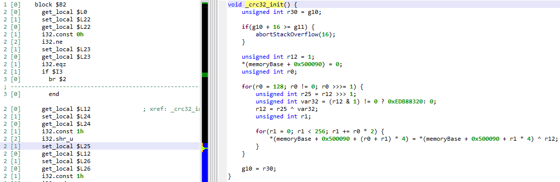
Let’s perform another decompilation of the same routine, with the unsafe optimizers enabled this time. GENDEC now will:
detect something that potentially could be decryption code
start emulating the underlying IR (not visible here, but you can easily read/write the Intermediate Representation via API) portion of code is emulated
collect and apply results
See the decrypted contents below. (An data item existed beforehand at 0x2F137, and the decompiler chose not to erase it.) The decompiled code on the right panel no longer shows the decryption loop: an optimizer has discarded it since it can no longer be executed.
Decompilation #2: unsafe optimizers enabled
We may convert the data item (or bytes) to a string by pressing the A key (menu Native, command Create String). The decompiled code will pick it up and refresh the AST as well.
The final result looks like:
The VM and decompiled view show the decrypted code, “ro.build.version.sdk”
A few additional comments:
This optimizer is considered unsafe3because it is allowed to modify the VM of the underlying native code unit, as seen above.
The optimizer is generic (architecture-agnostic). It performs its work on the underlying IR mid-stage in the decompilation pipeline, when various optimizations are applied.
It makes use of public API methods only, mostly the IREmulator class. Advanced users can write similar optimizers if they choose to. (We will also publish the code of this optimizer on GitHub shortly, as it will serve as a good real-life example of how to use the IR emulator to write powerful optimizers. It’s slightly more than 100 lines of Java.)
We hope you enjoy using JEB 4 Beta. There is a license type for everyone, so feel free to try things out. Do not hesitate to reach out to us on Twitter, Slack, or privately over email! Thanks, and until next time 🙂
Users familiar with JEB’s Dex decompilers will remember that a similar feature was introduced to JEB 3 in 2020, for Android Dalvik code. ↩
sha256 43816c47315aab27e50e6f895774a7b86d591807179e1d3262446ab7d68a56ef also available as lib/arm64-v8a/libd.so in 309d848275aa128ebb7e27e570e5a2876977122625638630a6c61f7434b771c3 ↩
“unsafe” in the context of decompilation; unsafe here is not to be understood as, “could any code be executed on the machine”, etc. ↩
Disclaimer: a long time ago in our galaxy, we published part 1 of this blog post; then we decided to wait for the next major release of JEB decompiler before publishing the rest. A year and a half later, JEB 4.0 is finally out! So it is time for us to publish our complete adventure with MarsAnalytica crackme. This time as one blog covering the full story.
In this blog post, we will describe our journey toward analyzing a heavily obfuscated crackme dubbed “MarsAnalytica”, by working with JEB’s decompiled C code 1.
To reproduce the analysis presented here, make sure to update JEB to version 4.0+.
Part 1: Reconnaissance
MarsAnalytica crackme was created by 0xTowel for NorthSec CTF 2018. The challenge was made public after the CTF with an intriguing presentation by its author:
My reverse engineering challenge ‘MarsAnalytica’ went unsolved at #nsec18 #CTF. Think you can be the first to solve it? It features heavy #obfuscation and a unique virtualization design.
Given that exciting presentation, we decided to use this challenge mainly as a playground to explore and push JEB’s limits (and if we happen to solve it on the road, that would be great!).
The MarsAnalytica sample analyzed in this blog post is the one available on 0xTowel’s GitHub2. Another version seems to be available on RingZer0 website, called “MarsReloaded”.
So, let’s examine the beast! The program is a large x86-64 ELF (around 10.8 MB) which, once executed, greets the user like this:
Inserting a dummy input gives:
It appears we have to find a correct Citizen ID! Now let’s open the executable in JEB. First, the entry point routine:
A few interesting imports: getchar() to read user input, and putchar() and puts() to write. Also, some memory manipulation routines, malloc() and memcpy(). No particular strings stand out though, not even the greeting message we previously saw. This suggests we might be missing something.
Actually, looking at the native navigation bar (right-side of the screen by default), it seems JEB analyzed very few areas of the executable:
Navigation Bar (green is cursor’s location, grey represents area without any code or data)
To understand what happened let’s first look at JEB’s notifications window (File > Notifications):
Notifications Window
An interesting notification concerns the “Initial native analysis styles”, which indicates that code gaps were processed in PROLOGUES_ONLY mode (also known as a “conservative” analysis). As its name implies, code gaps are then disassembled only if they match a known routine prologue pattern (for the identified compiler and architecture).
This likely explains why most of the executable was not analyzed: the control-flow could not be safely followed and unreferenced code does not start with common prologue patterns.
Why did JEB used conservative analysis by default? JEB usually employs aggressive analysis on standard Linux executables, and disassembles (almost) anything within code areas (also known as “linear sweep disassembly”). In this case, JEB went conservative because the ELF file looks non-standard (eg, its sections were stripped).
So, first a few memcpy() to copy large memory areas onto the stack, followed by series of “obfuscated” computations on these data. The main() routine eventually returns on an address computed in rax register. In the end, JEB disassembler was not able to get this value, hence it stopped analyzing there.
Let’s open the binary in JEB debugger, and retrieve the final rax value at runtime: 0x402335. We ask JEB to create a routine at this address (“Create Procedure”, P), and end up on very similar code. After manually following the control-flow, we end up on very large routines — around 8k bytes –, with complex control-flow, built on similar obfuscated patterns.
And yet at this point we have only seen a fraction of this 10MB executable… We might naively estimate that there is more than 1000 routines like these, if the whole binary is built this way (10MB/8KB = 1250)!
Most obfuscated routines re-use the same stack frame (initialized in main() with the series of memcpy()). In others words, it looks like a very large function has been divided into chunks, connected through each other by obfuscated control flow computations.
At this point, it seems pretty clear that a first objective would be to properly retrieve all native routines. Arguably the most robust and elegant way to do that would be to follow the control flow, starting from the entry point routine . But how to follow through all these obfuscated computations?
Explore The Code (At C Level)
Let’s now take a look at the pseudo-C code produced by JEB for those first routines. For example, here is main():
Decompiled main()
Overall, around 40 lines of C code, most of them being simple assignments, and a few others being complex operations. In comparison to the 200 non-trivial assembly instructions previously shown, that’s pretty encouraging.
What Do We Know
Let’s sum up what we noticed so far: MarsAnalytica’s executable is divided into (pretty large) handler routines, each of them passing control to the next one by computing its address. For that purpose, each handler reads values from a large stack, make a series of non-trivial computations on them, then write back new values into the stack.
As originally mentioned by 0xTowel, the crackme author, it looks like a virtual-machine style obfuscation, where bytecodes are read from memory, and are interpreted to guide the execution. It should be noted that virtual machine handlers are never re-executed: execution seems to go from lower to higher addresses, with new handlers being discovered and executed.
Also, let’s notice that while the executable is strongly obfuscated, there are some “good news”:
There does not seem to be any self-modifying code, meaning that all the code is statically visible, we “just” have to compute the control-flow to find it.
JEB decompiled C code looks (pretty) simple, most C statements are simple assignments, except for some lengthy expression always based on the same operations; the decompilation pipeline simplified away parts of the complexity of the various assembly code patterns.
There are very few subroutines called (we will come back on those later), and also a few system APIs calls, so most of the logic is contained within the chain of obfuscated handlers.
What Can We Do
Given all we know, we could try to trace MarsAnalytica execution by implementing a C emulator working on JEB decompiled code. The emulator would simulate the execution of each handler routine, update a memory state, and retrieve the address of the next handler.
The emulator would then produce an execution trace, and provide us access to the exact memory state at each step. Hence, we should find at some point where the user’s input is processed (typically, a call to getchar()), and then hopefully be able to follow how this input gets processed.
The main advantage of this approach is that we are going to work on (small) C routines, rather than large and complex assembly routines.
There are a few additional reasons we decided to go down that road:
– The C emulator would be architecture-independent — several native architectures are decompiled to C by JEB –, allowing us to re-use it in situations where we cannot easily execute the target (e.g. MIPS/ARM).
– It will be an interesting use-case for JEB public API to manipulate C code. Users could then extend the emulator to suit their needs.
– This approach can only work if the decompilation is correct, i.e. if the C code remains faithful to the original native code. In other words, it allows to “test” JEB decompilation pipeline’s correctness, which is — as a JEB’s developer — always interesting!
Nevertheless, a major drawback of emulating C code on this particular executable, is that we need the C code in the first place! Decompiling 10MB of obfuscated code is going to take a while; therefore this “plan” is certainly not the best one for time-limited Capture-The-Flag competitions.
Part 2: Building a (Simple) C Emulator
The emulator comes as a JEB back-end plugin, whose code can be found on our GitHub page. It starts in CEmulatorPlugin.java, whose logic can be roughly summarized as the following pseudo-code:
In this part we will focus on emulate()method. This method’s purpose is to simulate the execution of a given C routine from a given machine state, and to provide in return the final machine state at the end of the routine.
Decompiled C Code
First thing first, let’s explore what JEB decompiled code looks like, as it will be emulate() input. JEB decompiled C code is stored in a tree-structured representation, akin to an Abstract Syntax Tree (AST).
For example, let’s take the following C function:
int myfunction()
{
    int a = 1;
    while(a < 3) {
        a = a + 1;
    }
    return a;
}
The JEB representation of myfunction body would then be:
AST Representation (rectangles are JEB interfaces, circles are values)
As of JEB 4.0, the hierarchy of interfaces representing AST elements (i.e. nodes in the graph) is the following:
AST ICElement Hierarchy
Two parts of this hierarchy are of particular interest to us, in the context of building an emulator:
ICExpression represents C expressions, for example ICIdentifier (a variable), or ICOperation (any operation). Our emulator is going to evaluate those expressions, i.e. assign concrete values to them.
While an AST provides a precise representation of C elements, it does not provide explicitly the control flow. That is, the order of execution of statements is not normally provided by an AST, which rather shows how some elements contain others from a syntactic point-of-view.
In order to simulate a C function execution, we are going to need the control flow. So here is our first step: compute the control flow of a C method and make it usable by our emulator.
To do so, we implemented a very simple Control-Flow Graph (CFG), which is computed from an AST. The code can be found in CFG.java, please refer to the documentation for the known limitations.
Here is for example the CFG for the routine previously presented myfunction():
myfunction() CFG
Why does JEB does not provide a CFG for decompiled C code? Mainly because at this point JEB decompiler does not need it. Most important optimizations are done on JEB Intermediate Representation — for which there is indeed a CFG. On the other hand, C optimizations are mainly about “beautifying” the code (i.e. pure syntactic transformations), which can be done on the AST only 3.
Before digging into the emulation logic, let’s see how emulator state is represented and initialized.
Emulator State
The emulator state is a representation of the machine’s state during emulation; it mainly comprehends the state of the memory and of the CPU registers.
The memory state is a IVirtualMemory object — JEB interface to represent virtual memory state. This memory state is created with MarsAnalytica executable initial memory space (set by JEB loader), and we allocate a large area at an arbitrary address to use as the stack during emulation:
// initialize from executable memory
memory = nativeUnit.getMemory();

// allocate large stack from BASE_STACK_POINTER_DEFAULT_VALUE (grows downward)
VirtualMemoryUtil.allocateFillGaps(memory, BASE_STACK_POINTER_DEFAULT_VALUE - 0x10_0000, 0x11_0000, IVirtualMemory.ACCESS_RW);
The CPU registers state is simply a Map from register IDs — JEB specific values to identify native registers — to values:
Update the state according to the statement semantic, i.e. propagate all side-effects of the statement to the emulator state.
Determine which statement should be executed next; this might involve evaluating some predicates.
For example, let’s examine the logic to emulate a simple assignment like a = b + 0x174:
void evaluateAssignment(ICAssignment assign) {
  // evaluate right-hand side
  Long rightValue = evaluateExpression(assign.getRight());

  // assign to left-hand side
  state.setValue(assign.getLeft(), rightValue);
}
The method evaluateExpression() is in charge of getting a concrete value for a C expression (i.e. anything under ICExpression), which involves recursively processing all the subexpressions of this expression.
In our example, the right-hand side expression to evaluate is an ICOperation (b + 0x17). Here is the extract of the code in charge of evaluating such operations:
If b is a local variable, i.e. mapped in stack memory, the method ICIdentifier.getAddress() provides us its offset from the stack base address. Also note that an ICIdentifier has an associated ICType, which provides us the variable’s size (through the type manager, see emulator’s getTypeSize()).
Finally, evaluating constant 0x17 in the operation b + 0x17 simply means returning its raw value:
For statements with more complex control flow than an assignment, the emulator has to select the correct next statement from the CFG. For example, here is the emulation of a while loop wStm (ICWhileStm):
// if predicate is true, next statement is while loop body...
if(evaluateExpression(wStm.getPredicate()) != 0) {
   return cfg.getNextTrueStatement(wStm);
}
// ...otherwise next statement is the one following while(){..}
else {
   return cfg.getNextStatement(wStm);
}
In MarsAnalytica there are only a few system APIs that get called during the execution. Among those APIs, only memcpy() is actually needed for our emulation, as it serves to initialize the stack (remember main()). Here is the API emulation logic:
Long simulateWellKnownMethods(ICMethod calledMethod,
            List<ICExpression> parameters) {

        if(calledMethod.getName().equals("→time")) {
            return 42L; // value does not matter
        }
        else if(calledMethod.getName().equals("→srand")) {
            return 37L; // value does not matter
        }
        else if(calledMethod.getName().equals("→memcpy")) {
            ICExpression dst = parameters.get(0);
            ICExpression src = parameters.get(1);
            ICExpression n = parameters.get(2);
            // evaluate parameters concrete values
            [...REDACTED...]
            state.copyMemory(src_, dst_, n_);
            return dst_;
          }
       }
}
Demo Time
The final implementation of our tracer can be found in our GitHub page. Once executed, the plugin logs in JEB’s console an execution trace of the emulated methods, each of them providing the address of the next one:
Good news everyone: the handlers addresses are correct (we double-checked them with a debugger). In other words, JEB decompilation is correct and our emulator remains faithful to the executable logic. Phew…!
Part 3: Solving The Challenge
Plot Twist: It Does Not Work
The first goal of the emulator was to find where user’s input is manipulated. We are looking in particular for a call to getchar(). So we let the emulator run for a long time, and…
…it never reached a call to getchar().
The emulator was correctly passing through the obfuscated handlers (we regularly double-checked their addresses with a debugger), but after a few days the executed code was still printing MarsAnalytica magnificent ASCII art prompt (reproduced below).
MarsAnalytica Prompt
After investigating, it appears that characters are printed one by one with putchar(), and each of these calls is in the middle of one heavily obfuscated handler, which will be executed once only. More precisely, after executing more than one third of the whole 10MB, the program is still not done with printing the prompt!
As mentioned previously, the “problem” with emulating decompiled C code is that we need the decompiled code in the first place, and decompiling lots of obfuscated routines takes time…
Let’s Cheat
Ok, we cannot reach in a decent time the point where the user’s input is processed by the program. But the execution until this point should be deterministic. What if… we start the emulation at the point where getchar() is called, rather than from the entry-point?
In other words, we are going to assume that we “found” the place where user’s input starts to be processed, and use the emulator to analyze how this input is processed.
To do so, we used GDB debugger to set a breakpoint on getchar() and dumped both stack and heap memories at this point 5. Then, we extended the emulator to be able to initialize its memory state from stack/heap memory dumps, and change emulation start address to be the first call to getchar().
What Now?
At this point getchar() is called to get the first input character, so we let the emulator simulate this API by returning a pseudo-randomly chosen character, such that we can follow the rest of the execution. After 19 calls to getchar() we finally enter the place where user’s input is processed. Hooray…
Then, we let the emulator run for a whole day, which provided the execution trace we will be working on for the rest of this blog. After digging into the trace we noticed that input characters were passed as arguments to a few special routines.
Introducing The Stack Machine
When we first skimmed through MarsAnalytica code, we noticed a few routines that seemed specials for two reasons:
While obfuscated routines are executed only once and in a linear fashion (i.e. from low to high memory addresses), these “special” routines are at the very beginning of the executable and are called very often during the execution.
These routines’ code is not obfuscated and seems to be related with memory management at first sight.
For example, here is JEB decompiled code for the first of them (comments are ours):
long sub_400AAE(unsigned long* param0, int param1) {
    long result;
    unsigned long* ptr0 = param0;
    int v0 = param1;

    if(!ptr0) {
        result = 0xffffffffL;
    }
    else {
        // allocate new slot
        void* ptr1 = →malloc(16L);
        if(!ptr1) {
            /*NO_RETURN*/ →exit(0);
        }

        // set value in new slot
        *(int*)((long)ptr1 + 8L) = v0;

        // insert new slot in first position
        *(long*)ptr1 = *ptr0;
        *ptr0 = ptr1;
        result = 0L;
    }

    return result;
}
What we have here is basically a “push” operation for a stack implemented as a chained list (param0 is a pointer to the top of the stack, param1 the value to be pushed).
Each slot of the stack is 16 bytes, with the first 8 bytes being a pointer to the next slot and the next 4 bytes containing the value (remaining 4 bytes are not used).
It now seemed clear that these special routines are the crux of the challenge. So we reimplemented most of them in the emulator, mainly as a way to fully understand them. For example, here is our “push” implementation:
/** PUSH(STACK_PTR, VALUE) */
if(calledMethod.getName().equals("sub_400AAE")) {
    Long pStackPtr = evaluateExpression(parameters.get(0));
    Long pValue = evaluateExpression(parameters.get(1));

    long newChunkAddr = allocateNewChunk();

    // write value
    state.writeMemory(newChunkAddr + 8, pValue, 4);

    // link new chunk to existing stack
    Long stackAdr = state.readMemory(pStackPtr, 8);
    state.writeMemory(newChunkAddr, stackAdr, 8);

    // make new chunk the new stack head
    state.writeMemory(pStackPtr, newChunkAddr, 8);

}
Overall, these operations are implementing a custom data-structure that can be operated in a last-in, first-out fashion, but also with direct accesses through indexes. Let’s call this data structure the “stack machine”.
Here are the most used operators:
Address
Operator (names are ours)
Argument(s)
0x400AAE
PUSH
VALUE
0x4009D7
POP
VALUE
0x400D08
GET
INDEX
0x400D55
SET
INDEX,VALUE
Stack Machine’s Main Operators
Tracing The Stack Machine
At this point, we modified the emulator to log only stack operations with their arguments, starting from the first call to getchar(). The full trace can be found here, and here is an extract:
S: SET index:7 value:97
S: SET index:8 value:98
S: SET index:13 value:99
S: SET index:15 value:100
S: SET index:16 value:101

[...REDACTED...]

S: PUSH 2700
S: POP (2700)
S: SET index:32 value:2700
S: GET index:32
S: PUSH 2700
S: PUSH 2
S: POP (2)
S: POP (2700)
S: PUSH 2702

[...REDACTED...]
The trace starts with a long series of SET operations, which are storing the result of getchar() at specific indexes in the stack machine (97, 98, 99,… are characters provided by the emulator).
And then, a long series of operations happen, combining the input characters with some constant values. Some interesting patterns appeared at this point, for example:
S: POP (2)
S: POP (2700)
S: PUSH 2702
Here an addition was made between the two popped values, and the result was then pushed. Digging into the trace, it appears there are also handlers popping two values and pushing back a subtraction, multiplication, exclusive or, etc.
Another interesting pattern appears at several places:
S: POP (16335)
S: POP (1234764)
S: PUSH 1
Looking at the corresponding C code, it is actually a comparison between the two popped values — “greater than” in this case –, and the boolean result (0 or 1) is then pushed. Once again, different comparison operators (equal, not equal, …) are used in different handlers.
Finally, something suspicious also stood out in the trace:
S: PUSH 137
S: PUSH 99
S: POP (137)
S: POP (99)
The popped values do not match the order in which they were pushed!
Our objective here is to understand how input characters are manipulated, and what tests are done on them. In other words,we want to know for each POP/POP/PUSH pattern if it is an operation (and which operation — addition, subtraction …–), or a test (and which test — equal, greater than …–).
Again, note that routines implementing POP/POP/PUSH patterns are executed only once. So we cannot individually analyze them and rely on their addresses.
This is where working on decompiled C code becomes particularly handy. For each POP/POP/PUSH series:
We search in the method’s decompiled code if a C operator was used on the PUSH operand. To do so, it is as simple as looking at the operand itself, thanks to JEB decompiler’s optimizations! For example, here is a subtraction:
...
long v1 = pop(v0 - 0x65f48L);
long v2 = pop(v0 - 0x65f48L);
push(v0 - 0x65f48L, v1 - v2);
...
When a C operator is found in push() second operand, the emulator adds the info (with the number of operands) in the trace:
S: POP (137)
S: POP (99)
S: PUSH 38
| operation: (-,#op=2)
Also, we check if there is a “if” statement following a POP in the C code. For example, here is a “greater-than” check between popped values:
...
long v2 = pop(v0 - 0x65f48L);
long v3 = pop(v0 - 0x65f48L);
if(v2 > v3) {
...
If so, the emulator extracts the C operator used in the if statement and logs it in the trace (as a pseudo stack operator named TEST):
S: POP (16335)
S: POP (1234764)
S: TEST (>,#op=2)
S: PUSH 0
It should be noted that operands are always ordered in the same way: first poped value is on left side of operators. So operators and operands are the only thing we need to reconstruct the whole operation.
Time To Go Symbolic
At this point, our execution trace shows how the user’s input is stored onto the stack, and which operations and tests are then done. Our emulator is providing a “bad” input, so they are certainly failed checks in our execution trace. Our goal is now to find these checks, and then the correct input characters.
At this point, it is time to introduce “symbolic” inputs, rather than using concrete values as we have in our trace. To do so, we made a quick and dirty Python script to replay stack machine trace using symbolic variables rather than concrete values.
First, we initialize a Python “stack” with symbols (the stack is a list(), and the symbols are strings representing each character “c0“, “c1“, “c2“…). We put those symbols at the same indexes used by the initial SET operations:
# fill stack with 'symbolic' variables (ie, characters)
# at the initial offset retrieved from the trace
stack = [None] * 50 # arbitrary size
charCounter = 0
stack[7] = 'c' + str(charCounter) # S: SET index:7 value:c0
charCounter+=1
stack[8] = 'c' + str(charCounter) # S: SET index:8 value:c1

[... REDACTED ...]
We also need a temporary storage for expressions that get popped from the stack.
Then, we read the trace file and for each stack operation we execute the equivalent operation on our Python stack:
if operator == "SWAP":
  last = stack.pop()
  secondToLast = stack.pop()
  stack.append(last)
  stack.append(secondToLast)

elif operator == "GET":
  index = readIndexFromLine(curLine)
  temporaryStorage.append(stack[int(index)])

elif operator == "SET":
  index = readIndexFromLine(curLine)
  stack[int(index)] = temporaryStorage.pop()

elif operator == "POP":
  value = stack.pop()
  temporaryStorage.append(value)

[... REDACTED ...]
Now here is the important part: whenever there is an operation, we build a new symbol by “joining” the symbol operands and the operator. Here is an example of an addition between symbols “c5” and “c9“, corresponding respectively to the concrete input characters initially stored at index 26 and 4:
Concrete Trace
Symbolic Trace
...
GET index:26

PUSH 102

GET index:4

PUSH 106

POP (106)

POP (102)

PUSH 208
  | operation: (+,#op=2)
...
...
GET index:26

PUSH "c5"

GET index:4

PUSH "c9"

POP ("c9")

POP ("c5")

PUSH "c9+c5"

...
Concrete execution trace, and its corresponding symbolic trace; on the symbolic side, rather than pushing the actual result of 106 + 102, we build an addition between the two symbols corresponding to the two concrete values
Note that our symbolic executor starts with a clean stack, containing only input symbols. All constants used during the computation are indeed coming from the bytecode (the large memory area copied on the (native) stack at the beginning of the execution), and not from the stack machine.
We can then observe series of operations on input symbols getting build by successive POP/POP/PUSH patterns, and being finally checked against specific values. Here is an extract of our stack at the end:
Here is another advantage to work with C code: the expressions built from our emulator’s trace are using high-level operators, which are directly understood by Z3.
Finally, we ask Z3 for a possible solution to the constraints, and we build the final string from c0, c1,… values:
m = s.model()
result = ''
result += chr(m[c0].as_long())
result += chr(m[c1].as_long())
result += chr(m[c2].as_long())
result += chr(m[c3].as_long())
...
And…
Hurray!
Conclusion
We hope you enjoy this blog post, where we used JEB C decompiled code to analyze a heavily obfuscated executable.
Please refer to our GitHub page for emulator code. While it has been tailored for MarsAnalytica crackme, it can be extended to emulate any executable’s decompiled C code (MarsAnalytica’s specific emulation logic is constrained in subclass MarsAnalyticaCEmulator).
You can run the plugin directly from JEB UI (refer to README):
By default, it will show emulation traces as text subunits in JEB project (stack machine trace in MarsAnalytica mode, or just C statements trace):
Plugin output: left panel is MarsAnalytica stack machine trace (when MarsAnalytica specific emulation logic is enabled), while right panel shows C statements emulation trace
Alternatively, the plugin comes with a headless client, more suitable to gather long running emulation traces.
Finally, kudo to 0xTowel for the awesome challenge! You can also check the excellent Scud’s solution.
Feel free to message us on Slack if you have any questions. In particular, we would be super interested if you attempt to solve complex challenges like this one with JEB!
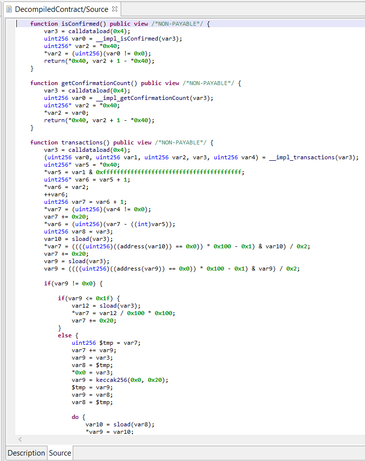
While JEB’s default decompiled code follows (most of) C syntactic rules and their semantics, some custom operators might be inserted to represent low-level operations and ease the reading; hence strictly speaking JEB’s decompiled code should be called pseudo-C. The decompiled output can also be variants of C, e.g. the Ethereum decompiler produce pseudo-Solidity code. ↩
SHA1 of the UPX-packed executable: fea9d1b1eb9d3f93cea6749f4a07ffb635b5a0bc ↩
Implementing a complete CFG on decompiled C code will likely be done in future versions of JEB, in order to provide more complex C optimizations. ↩
The actual implementation is more complex than that, e.g. it has to deal with pointers dereferencement, refer to emulateStatement() for details. ↩
Dumping memory was done with peda for GDB, and commands dumpmem stack.mem stack and dumpmem heap.mem heap↩
The third part of this series is about bytecode virtualization. The analyses that follow were done statically.
Bytecode virtualization is the most interesting and technically challenging feature of this protector.
TL;DR: – JEB Pro can un-virtualize protected methods. – A Global Analysis (Android menu) will point you to p-code VM routines. – Make sure to disable Parse Exceptions when decompiling such methods. – For even clearer results, rename opaque predicates of the method to guard0/guard1 (refer part 1 of this blog for details)
What Is Code Virtualization
Relatively novel, code virtualization is possibly one of the most effective protection technique there is 1. With it come relatively heavy disadvantages, such as hampered speed of execution 2 and the difficulty to troubleshoot production code. The advantages are heightened reverse-engineering hurdles over other more traditional software protection techniques.
Virtualization in the context of code protection means:
Generating a virtual machine M1
Translating an original code object C0 meant to be executed on a machine M03, into a semantically-equivalent code object C1, to be run on M1.
While the general features of M1 are likely to be fixed (e.g., all generations of M1 are stack machines with such and such characteristics), the Instruction Set Architecture (ISA) of M1 may not necessarily be. For example, opcodes, microcodes and their implementation may vary from generation to generation. As for C1, the characteristics of a generation are only constrained by the capabilities of the converter. Needless to say, standard obfuscation techniques can be applied on C1. The virtualization process can possibly be recursive (C1 could be a VM implementing the specifications of a machine M2, executing a code object C2, emulating the original behavior of C0, etc.).
All in all, in practice, this makes M1 and C1 unique and hard to reverse-engineer.
Before and after virtualization of a code object C0 into C1
Example of a Protected Method
Note: all identifier names had been obfuscated. They were renamed for clarity and understanding.
Below, the class VClass was found to be “virtualized”. A virtualized class means that all non-constructor (all but <init>(*)V and <clinit>()V) methods were virtualized.
Interestingly, the constructors were not virtualized
The method d(byte[])byte[] is virtualized:
It was converted into an interpreter loop over two large switch constructs that branch on pseudo-code entries stored in the local array pcode.
A PCodeVM class was added. It is a modified stack-based virtual machine (more below) that performs basic load/store operations, custom loads/stores, as well as some arithmetic, binary and logical operations.
Virtualized method. Note the pcode array. The opcode handlers are located in two switches. This picture shows the second switch, used to handle specific operations and API calls.
A snippet of the p-code VM class. Full code here, also contains the virtualized class.
The generic interpreter is called via vm.exec(opcode). Execution falls back to a second switch entry, in the virtualized method, if the operation was not handled.
Please refer to the gist linked above for a full list of “generic” VM operations. Three examples, including one showing that the operations are not as generic as the term implies:
(specific to this VM) opcode 6, used to peek the most recently pushed object(specific to this VM) opcode 8, a push-int operation(specific to this VM) opcode 23 is relatively specialized, it implements an add-xor stack operation (pop, pop, push). It is quite interesting to see that the protection system does not simply generate one-to-one, dalvik-to-VM opcodes. Instead, the target routine is thoroughly analyzed, most likely lifted, high-level (compounded) arithmetic operations isolated, and pseudo-generic (in PCodeVM) or specialized (in the virtualized method) opcodes generated.
As said, negative opcodes represent custom operations specific to a virtualized method, including control flow changes. An example:
opcode -25: a if(a >=b) goto LABEL operation (first, call into opcode 55 to do a GE operation on the top two integers; then, use the result to do conditional branching)
Characteristics of the P-code VM
From the analysis of that code as well as virtualized methods found in other binaries, the characteristics of the p-code VM generated by the app protector can be inferred:
The VM is a hybrid stack machine that uses 5 parallel stacks of the same height, stored in arrays of:
java.lang.Object (accommodating all objects, including arrays)
int (accommodating all small integers, including boolean and char)
long
float
double
For each one of the 5 stack types above, the VM uses two additional registers for storing and loading
Two stack pointers are used: one indicates the stack TOP, the other one seems to be used more liberally, and is akin to a peek register
The stack has a reserved area to store the virtualized method parameters (including this if the method is non-static)
The ISA encoding is trivial: each instruction is exactly one-word long, it is the opcode of the p-code instruction to be executed. There is no concept of register, index, or immediate value embedded into the instruction, as most stack machine ISA’s have.
Because the ISA is so simple, the implementation of the semantics of an instruction falls almost entirely on the p-code handler. For this reason, they were grouped into two categories:
Semi-generic VM operations (load/store, arithmetic, binary, tests) are handled by the VM class and have a positive id. (A VM object is used by every virtualized method in a virtualized class.)
Operations specific to a given virtualized method (e.g., method invocations) use negative ids and are handled within the virtualized method itself.
While the PCodeVM opcodes are all “useful”, many specific opcodes of a virtualized method (negative ids) achieve nothing but the execution of code semantically equivalent to NOP or GOTO.
opcodes -2, -1: essentially branching instructions. A substantial amount of those can be found, including some branching to blocks with no other input but that source (i.e., an unnecessary GOTO – =spaghetti code -, or a NOP operation if the next block is the follow.)
Rebuilding Virtualized Methods
Below, we explain the process used to rebuild a virtualized method. The CFG’s presented are IR-CFG’s (Intermediate Representations) used by the dexdec4 pipeline. Note that unlike gendec‘s IR 5, dexdec‘s IR is not exposed publicly, but its textual representation is mostly self-explanatory.
Overall, a virtualized routine, once processed by dexdec like any other routine, looks like the following: A loop over p-code entries (stored in x8 below), processed by a() at 0xE first, or by the large routine switch.
Virtualized method, optimized, virtualized
The routine a() is PCodeVM.exec(), and its optimized IR boils down to a large single switch. 6
PCodeVM.exec()
The unvirtualizer needs to identify key items in order to get started, such as the p-code entries, identifiers used as indices into the p-code array, etc. Once they have been gathered, concolic execution of the virtualized routine becomes possible, and allows rebuilding a raw version of the original execution flow. Multiple caveats need to be taken care of, such as p-code inlining, branching, or flow termination. In its current state, the unvirtualizer disregards exceptional control flow.
Below, a raw version of the unflattened CFG. Note that all operations are stack-based; the code itself has not been modified at this point, it still consists of VM stack-based operations.
Virtualized method after unflattening, raw
dexdec’s standard IR optimization passes (dead-code removal, constant and variable propagation, folding, arithmetic simplification, flow simplifications, etc.) clean up the code substantially:
Virtualized method after unflattening and IR optimizations (opt1)
At this stage, all operations are stack-based. The high-level code generated from the above would be quite unwieldy and difficult to analyze, although substantially better than the original double-switch.
The next stage is to analyze stack-based operations to recover stack slots uses and convert them back to identifiers (which can be viewed as virtual registers; essentially, we realize the conversion of stack-based operations into register-based ones). Stack analysis can be done in a variety of ways, for example, using fixed-point analysis. Again, several caveats apply, and the need to properly identify stacks as well as their indices is crucial for this operations.
Virtualized method after unflattening, IR optimizations, VM stack analysis (opt2)
After another round of optimizations:
Virtualized method after unflattening, IR optimizations, VM stack analysis, IR optimizations (opt2_1)
Once the stack analysis is complete, we can replace stack slot accesses by identifier accesses.
Virtualized method after unflattening, IR optimizations, VM stack analysis, IR optimizations, virtual registers insertion (opt3)
After a round of optimizations:
Virtualized method after unflattening, IR optimizations, VM stack analysis, IR optimizations, virtual registers insertion, IR optimizations (opt3)
At this point, the “original” CFG is essentially reconstructed, and other advanced deobfuscation passes (e.g., emulated-based deobfuscators) can be applied.
The high-level code generation yields a clean, unvirtualized routine:
High-level code, unvirtualized, unmarked
After reversing, it appears to be a modified RC4 algorithm. Note the +3/+4 added to the key.
High-level code, unvirtualized, marked
Detecting Virtualized Methods
All versions of JEB detect virtualized methods and classes: run Global Analysis (GUI menu: Android) on your APK/DEX and look for those special events:
JEB Pro version 3.22 7 ships with the unvirtualizer module.
Tips:
Make sure to enable the Obfuscators, and enable Unvirtualization (enabled by default in the options).
The try-blocks analysis must be disabled for the class to unvirtualize. (Use MOD1+TAB to redecompile, untick “Parse Exception Blocks”).
After a first decompilation pass, it may be easier to identify guard0/guard1, rename, and recompile, else OP obfuscation will remain and make the code unnecessarily difficult to read. (Refer to part 1 of this series to learn about what renaming those fields to those special names means and does when a protected app is detected.)
Conclusion
We hope you enjoyed this third installment on code (un)virtualization.
There may be a fourth and final chapter to this series on native code protection. Until next time!
—
On a personal note, my first foray into VM-based protection dates back to 2009 with the analysis of Trojan.Clampi, a Windows malware protected with VMProtect ↩
Although one could argue that with current hardware (fast x64/ARM64 processors) and software (JIT’er and AOT compilers), that drawback may not be as relevant as it used to be. ↩
Machine here may be understood as physical machine or virtual machine ↩
Note the similarities with CFG flattened by chenxification and similar techniques. One key difference here is that the next block may be determined using the p-code array, instead of a key variable, updated after each operation. I.e., is the FSM – controlling what the next state (= the next basic block) is – embedded in the flattened code itself, or implemented as a p-code array. ↩
JEB Android and JEB demo builds do not ship the unvirtualizer module. I initially wrote this module as a proof-of-concept not intended for release, but eventually decided to offer it to our professional users who have legitimate (non malicious) use cases, e.g. code audits and black-box assessments. ↩
Last week we presented a talk at REcon on the internals of JEB’s native disassembler.
During this talk, we focused on some of the research problems we encountered while developing our custom disassembler engine — the foundation for JEB native decompiler.
As the latest update makes its way to all users (changelog), it is a good time to quickly recap additions related to Android analysis that made it into JEB versions 3.1.4, 3.1.5, and 3.2.
Dalvik Decompiler Updates
The newest releases of JEB contain several improvements to the Dalvik decompiler. I will highlight only a couple that users may find interesting. 1
Enumerations
Compiled Java enumerations can be complicated beasts. JEB attempts to re-sugar them to the best of its ability. On failure, regular classes extending java.lang.Enum will be rendered.
Obfuscation sometimes destroy important synthetic fields and structures that allow recovery heuristics to work. However, support should function reasonably well, even on enumeration data that was intentionally shuffled to generate decompilation errors. Moreover, and to keep with the spirit of interactivity in JEB, enumerated fields can be renamed – and it is done consistently over the code base, including over reconstructed switches making use of such enums.
Decompiled enums in android.arch.lifecycle. Renaming and cross-referencing enumerated constants is supported.
Custom enumerated constants are also properly reconstructed, including:
Field annotations
Custom initializers (see below)
Additional methods and method overrides
In this complex enumeration, the red block shows a custom initializer. Other interesting bits are the use of overrides and custom methods, annotations, as well as default and non-default constructors.
Switches
Support was recently added for switch-on-enum and switch-on-string (partial support for the latter, to be continued in the next software update).
This successfully reconstructed switch-on-string is implemented as a double-switch idiom by dx (a sparse switch on hashCode/equals to generate custom indices i, followed by a packed-switch on i). Not all switches are implemented like this. Regular if-conditional trees may be strategically generated by optimizing compilers.
Inner classes, Anonymous classes
We improved rendering support for named- and anonymous-inner classes. Properly rendering anonymous classes in particular is made difficult by the fact that some of its arguments are captured from the outer classes. Properly rendering anonymous constructors, with exact argument types and position, is also challenging.
Lately, a user sent us a sample making use of an anonymous class initializer to hide string decryption code. See below:
The anonymous class extends Android’s OnActivityResultListener, instantiates the object, and tosses it immediately.
Decryption code takes place in the initializer. Note the captured arguments from the outer container method __m: i, _b. Access to other private class fields is made via synthetic accessor calls that were re-sugared into seemingly direct field access (BA._b).
Pseudo-moot anonymous class with an instance initializer attempting to conceal string decryption code.
Plugin options
Remember that some decompiler properties are publicly available in the options: (menu: Edit, Options, Advanced, Engines)
All Dalvik decompilation options: see the .parsers.dcmp_dex.* namespace
All Java rendering options of decompiled code: see the .parsers.dcmp_dex.text.* namespace
1)Rendering options are real-time options that can be changed after the fact to customize the output. Right-click on a decompiled class output, and select Rendering Options:
2) Decompilation options are used to guide and customize the decompilation. They can be changed in the Engines options, or more simply, when performing a decompilation itself, by invoking “Decompile with Options…” instead of “Decompile”.
Keyword for “Decompile with Options”: CTRL+TAB (Windows, Linux) or COMMAND+TAB (macOS)
Bring up the “Decompile with Options” dialog by using CTRL+TAB/COMMAND+TAB when decompiling. Hover over properties to get extra documentation in the tooltip.
API additions
Essential updates to:
IJavaSwitch: additional methods to access switch-on-enum and switch-on-string data
IJavaForEach: additional type introduced to manipulate for-each statements: for(Type var: iterator_or_array) { … }
Other changes, What next
JEB 3.2 contains other improvements, such as:
Better auto-naming, including default usage of debug data, if present (can be disabled in the options)
Improved typing and type propagation
Additional IR and AST optimizations
Better exceptional flow processing
Rendering of try-catch, synchronized blocks, etc.
Decompilation of invoke-polymorphic (invoke-custom is not supported, see below the part on lambdas on method handles)
We have more planned for the coming releases, including:
Improved support for switch-on-string. As said earlier, some of those switches, when properly detected, are re-sugared into legal Java-8 switch-on-string. However, the nature of those high-level constructs (they are implemented as double-conditionals, sometimes double-switches) makes it quite hard in some cases to provide proper reconstruction. It is something that will be improved in the future.
Support for generics. We had decided to not implement Java 5-style type generic since the information, when provided, is stored as pure metadata and should not be trusted. However, in practice, it turns out to be helpful when auditing legitimate, non-obfuscated compiled apps. We will add optional support for that in a coming release.
Support for try-with-resources.try(resource)/catch/finally are difficult very-high-level idioms to reconstruct. Optimizing compilers generate a substantial amount of additional, highly optimized code to implicitly catch exceptions and auto-close resources, making it extra difficult to reconstruct in the general case. We will likely introduce partial support before the summer.
Lambdas. It is a planned addition. We will soon be re-sugaring Android implementations of Java 8+ lambdas into proper lambda functions. Same goes for method handles (::). That’s quite exciting and may pave the way for a hypothetical Kotlin decompiler, since that language implicitly and explicitly rely on lambdas extensively.
Debuggable APK Generation
For several reasons, it is easier to debug Android applications explicitly marked debuggable in their Manifest.
Debugging non-debuggable APK requires root access to the operating system. Which means rooting a production phone, using an emulator 2 image built as userdebug, or building a custom userdebug image from AOSP.
Any of the above solutions have shortcomings: rooted production builds and userdebug builds expose features that non-rooted production builds do not have, and can be fingerprinted as such; Debugging native code of applications on non-rooted devices requires replacing system-level utilities; the API level and OS features also play a role, eg, SE-Android needs to be disabled on recent OS in order for debugging to work.
In many cases, rebuilding a release app into a debug-mode app (with <application android:debuggable=”true” …>) is a viable solution, and one that does not require using root, obviously. Many users are implementing this solution via apktool. However it is frequent for the tool to fail decoding complex APKs, let alone rebuild them with different settings.
We have introduced a feature in JEB that makes rebuilding non-debuggable APK to debuggable APK easy and fast:
$ jeb_wincon.bat -c --makeapkdebug -- file.apk
Upon success, file_debuggable.apk will be generated. Sign it (Android SDK’s apksigner), install it on your device, and start debugging. Remember that this solution has its shortcomings as well! Anti-debugging code may check at runtime that the app is not debuggable, as would be expected. More elaborate solutions implement certificate pinning-style checks, where the code verifies that it is signed using a specific certificate. Be careful when debugging rebuilt APK.
This malware app was made debuggable
Keyboard Shortcuts for Script
Bind your JEB Python scripts to keyboard shortcut by adding a line at the top of your script:
#?shortcut=xxx
where xxx is your keyboard shortcut, eg: Ctrl+Shift+T
Permitted keyboard modifiers are Ctrl, Shift, Alt, as well as the generic Mod1, mapping to macOS’s Command (Apple) key, or Control on Windows/Linux.
Sublime Text 3 Extension
Are you writing Python scripts to automate your JEB reversing tasks? If so, give a try to using the “JEB Script Development Helper” package available on Sublime Text’s Package Control.
In part 1 of this series, we gave an overview of the Intermediate Representation used by JEB’s Native Analysis Pipeline, as well as a simple Python script demonstrating how to use the API to access and print out IR-CFG of decompiled routines.
In part 2, we continue our exploration of JEB IR. We will show how to write a custom IR optimizer plugin to clean-up a custom obfuscation used in a piece of code. The resulting decompiled C code will end up very readable as well.
Before you proceed, make sure to update JEB Pro to version 3.1.1+.
Obfuscated Crypto-stealer Code
The sample we are going to look at monitors Windows clipboards for cryptocurrency-looking wallet addresses, and replaces them with a desired target address. The sample is specifically targeting Ethereum wallet addresses. It is a neutered final stage payload – the recipient address has been scrambled to render the code ineffective.
PE characteristics of file 1.exe
Although the payload is unpacked, what is interesting is that one of its key routines is obfuscated: custom garbage code was inserted.
Junk (useless) assignments
The garbage code is easy to go through: a bit of manual analysis shows that junk instructions are assigning pseudo-random values to an array whose bytes are never used. Two types of assembly patterns are present:
1- mov dword ptr [edi + offset], junk_value ; edi previously init. to
                                            ; junkarray address
2- push junk_value
   pop dword ptr [junkarray_address + offset]
If we decompile that code and look at the final IR (as shown below), we can see that those instructions ended up being converted and optimized to the following type of assignment:
Assign(Mem(mem_address), Imm(junk_value))
Currently, the decompiled code looks like the following, hard-to-digest blob:
Snippet of decompiled code (obfuscated)
Although quite painful to read, we can follow the program’s logic by abstracting away the junk assignments. (Essentially, win32 functions’ OpenClipboard, GetClipboardData, and SetClipboardData are used to retrieve, check, and replace copy-pasted Ascii and Unicode text, if they match the following pattern “/0x(..){20}/”. The replacement string target wallet address, previously decrypted by sub_401000.)
Cleaning the Intermediate Representation
Recall that the native analysis pipeline can be simplifed as the workflow below:
CodeObject (*) -> Reconstructed Routines & Data -> Conversion to IR (low-level, non-optimized) -> IR Optimizations<--- this is where we'll work -> Final IR (higher-level, optimized, typed) -> Generation of AST -> AST Optimizations -> Final AST (final, cleaned) -> High-level output (eg, C variant)
Our custom IR optimizer will look for junk assignments and remove them. The important criteria are: What is the junk array start and end addresses? Is it common to all routines in the binary, or is there one array per routine? Those questions may be hard to answer in the general case. However, for our specific sample file, we can assert with a high-degree of certainty that the junk array: – starts at address 0x415882 – is at most 256 bytes long – is used solely by sub_401171, the routine we want to analyze
Because of the above restrictions, the IR optimizer we are going to write should be qualified as a custom or ad-hoc IR optimizer. Chances are, we won’t be able to reuse it as-is in other programs without some amount of tweaking.
Let’s get started, we will: – create an Eclipse project with scaffold code for a Java back-end plugin – write and test a custom IR optimizer with a headless client – deploy the plugin and make it usable and accessible from the UI desktop client
Creating a Plugin Project
Before we proceed, make sure to:
Define an environment variable JEB_HOME, that points to your JEB installation folder
Open Eclipse and import the newly-created project into your Workspace (File, Import, Existing Projects into the Workspace, select the cloned repository folder, proceed)
Importing an existing project into Eclipse
Debugging the Obfuscation
Now that your project is imported in Eclipse, you should be able to see two source files in src’s default package:
Tester.java
EOptExample1.java
EOptExample1 is the IR optimizer plugin we will be working on. (Note that several classes of plugins exist, this one is a native IR optimizer, and therefore inherits from AbstractEOptimizer or one its subclasses.)
Tester creates a headless JEB instance that loads the plugin EOptExample1.
Package Explorer view of the newly-created project
Then, create a JEB project and load the artifact file samples/1.exe (IMPORTANT: unzip 1.zip to 1.exe first – password: password)
Analyze the artifact
Retrieve a handle on the native decompiler
Retrieve a handle on the to-be-analyzed routine sub_401171
Perform a full decompilation of that routine
Let’s have a preliminary look at EOptExample1: This IR optimizer type is set to STANDARD, which is not ideal when you use custom optimizers tailored for specific code. A better IR optimizer class for those is ON_DEMAND: those optimizers are to be manually invoked, e.g. from JEB UI (menu: File, Advanced Unit Options). However, during development, since we are focusing on a particular file and routine, STANDARD type may be fine. Standard optimizers are called during regular IR optimization phases of the decompilation pipeline.
public class EOptExample1 extends AbstractEOptimizer {

    public EOptExample1() {
        super(DataChainsUpdatePolicy.UPDATE_IF_OPTIMIZED);
        getPluginInformation().setName("Sample IR Optimizer #1");
        getPluginInformation().setDescription("Remove IR-statements reduced to \"*(&garbage + delta) = xxx\"");
        getPluginInformation().setVersion(Version.create(1, 0, 0));
        // Standard optimizers are normally run, as part of the IR optimization stages in the decompilation pipeline
        setType(OptimizerType.STANDARD);
    }

    // replace all IR statements previously reduced to EMem ("[junk_address] = xxx") to ENop
    @Override
    public int perform(boolean updateDFA) {
        logger.info("IR-CFG before running custom optimizer \"%s\":\n%s", getName(),
                DecompilerUtil.formatIRCFGWithContext(2, cfg, ectx));
        // ...
        // optimizer code
    }
}
Note the plugin’s data-chains update policy, set to UPDATE_IF_OPTIMIZED. Optimizations that specify this flag tell their runner, aka the master optimizer that orchestrate them, that identifiers may be modified – hence, if optimizations occurred, a data flow analysis (DFA) pass needs to take place again. DFA update policies are a topic for another article.
Lines 3-5 are plugin metadata information, such as name and description, authorship, version numbers (including minimum/maximum JEB back-end versions), etc.
Before we deep-dive into perform(), let’s first set a breakpoint on line 15, where logger.info(…) is called. Then, start a debugging session for Tester: menu Run, command Debug (hotkey: F11.)
After a few seconds of analysis, your breakpoint should be hit; it corresponds to the first-time invocation of your custom optimizer. The logger prints out the IR-CFG that’s about to be optimized. Let’s have a look at it:
IR-CFG before running custom optimizer "Sample IR Optimizer #1":
>> IN(@0): ecx={@D} esp={@0} ebp={@1} ss={@1,@C,@18,@1D,@21,@24,@25,@27,@30,@35,@38,@3B,@3E,@3F,@41,@43,@46,@4F,@51,@54,@56,@59,@5C,@5D,@5F,@6B,@77,@81,@84,@9B,@9E,@A0,@AC,@B8,@BA,@BD,@BF,@C3,@C5,@C7,@CB,@CD,@D1,@D2,@D4,@E0,@E9,@EF,@F1,@F5,@F7,@FB,@FC,@FE,@100,@103,@106,@107,@109,@10C,@10E,@112,@114,@116,@11A,@11C,@11F,@122,@123,@12E,@131,@133,@137,@139,@13D,@13E,@140,@143,@145,@149,@14B,@14F,@150,@152,@15D,@173,@176,@179,@17C,@17D,@17F,@181,@18A,@18C,@18F,@191,@194,@196,@19A,@19D,@19E,@1A0,@1B3,@1BF,@1C2,@1D9,@1DC,@1E0,@1EC,@1EF,@1F1,@1F3,@1F7,@1F9,@1FC,@1FF,@202,@203,@205,@211,@21D,@220,@222,@226,@227,@229,@22B,@22E,@231,@232,@234,@237,@23A,@23C,@23E,@242,@244,@246,@24A,@24C,@250,@251,@25C,@25F,@262,@263,@265,@268,@26A,@26E,@271,@272,@27A,@27F,@295,@298,@29A,@29D,@2A4,@2A9,@2AD,@2B0,@2B2,@2B6,@2B7,@2BA,@2BC,@2C0,@2C2,@2C6,@2C7,@2CA,@2CD,@2D2,@2DE,@2E4,@2E7,@2E8,@2EA} ds={@F,@11,@19,@1E,@22,@28,@31,@36,@39,@3C,@40,@44,@4C,@4E,@52,@55,@57,@5A,@60,@6C,@74,@78,@7B,@82,@85,@86,@87,@8E,@90,@92,@9C,@A1,@A3,@A4,@AD,@B5,@B7,@BB,@C0,@C4,@C8,@CE,@D5,@E1,@EA,@ED,@F2,@F8,@FD,@FF,@101,@104,@10A,@10F,@113,@117,@11B,@11D,@120,@124,@12F,@134,@13A,@13F,@141,@146,@14C,@153,@15A,@15C,@163,@165,@166,@167,@170,@171,@174,@177,@17A,@17E,@180,@187,@189,@18D,@192,@197,@19B,@1A1,@1AB,@1B4,@1B7,@1B9,@1C0,@1C3,@1C4,@1C5,@1CC,@1CE,@1D0,@1DA,@1DD,@1DE,@1E1,@1E9,@1ED,@1F0,@1F4,@1FA,@1FD,@200,@206,@212,@219,@21B,@21E,@223,@228,@22A,@22C,@22F,@235,@238,@23B,@23F,@243,@247,@24D,@252,@25B,@25D,@260,@264,@266,@26B,@26F,@273,@27B,@27E,@285,@287,@288,@289,@292,@293,@296,@29B,@2A5,@2AA,@2AE,@2B3,@2B8,@2BD,@2C3,@2C8,@2CE,@2D0,@2D3,@2DF,@2E1,@2E2,@2E5,@2EB} OpenClipboard={@25} GetClipboardData={@3F,@17D} GlobalAlloc={@FC,@227} GlobalLock={@107,@232} GlobalUnlock={@13E,@263} SetClipboardData={@150,@272,@2B7,@2C7} CloseClipboard={@2CB} Sleep={@2E8} sub_401000={@D} sub_405010={@5D} sub_404F80={@D2} sub_4024E0={@123,@251} sub_404E54={@19E} sub_404E14={@203}
0000/1>  s32:_esp = (s32:_esp - i32:00000004h)                                                                 DU: esp={@1,@2,@B}                 | UD: esp={}
0001/1:  32<s16:_ss>[s32:_esp] = s32:_ebp                                                                      DU:                                | UD: esp={@0} ebp={} ss={}
0002/9:  s32:_ebp = s32:_esp                                                                                   DU: ebp={@38,@41,@46,@4F,@54,@56,@84,@9E,@B8,@BD,@C5,@FE,@100,@10C,@114,@11C,@131,@140,@15D,@176,@17F,@181,@18A,@18F,@194,@1C2,@1DC,@1EF,@1F1,@1FC,@229,@22B,@237,@23C,@244,@25C,@265,@27F,@298,@29D}  | UD: esp={@0}
000B/1:  s32:_esp = (s32:_esp - i32:0000002Ch)                                                                 DU: esp={@C,@D,@17}                | UD: esp={@0}
000C/1:  32<s16:_ss>[s32:_esp] = i32:0040117Ch                                                                 DU:                                | UD: esp={@B} ss={}
000D/1:  call s32:_sub_401000(s32:_ecx)->(s32:_eax){32[s32:_esp]}                                              DU: eax={}                         | UD: ecx={} esp={@B} sub_401000={}
000E/1+  s32:_edi = i32:00415882h                                                                              DU: edi={}                         | UD:
000F/1:  32<s16:_ds>[i32:00415944h] = i32:E2E60682h                                                            DU:                                | UD: ds={}
0010/1:  s32:_eax = i32:00000001h                                                                              DU: eax={}                         | UD:
0011/6:  32<s16:_ds>[i32:00415904h] = i32:7C64C0E4h                                                            DU:                                | UD: ds={}
0017/1:  s32:_esp = (s32:_esp - i32:00000004h)                                                                 DU: esp={@18,@1A}                  | UD: esp={@B,@2EC}
0018/1:  32<s16:_ss>[s32:_esp] = i32:E87A1612h                                                                 DU:                                | UD: esp={@17} ss={}
0019/1:  32<s16:_ds>[i32:004158DDh] = i32:E87A1612h                                                            DU:                                | UD: ds={}
001A/1:  s32:_esp = (s32:_esp + i32:00000004h)                                                                 DU: esp={@1C}                      | UD: esp={@17}
001B/1:  nop                                                                                                   DU:                                | UD:
001C/1+  s32:_esp = (s32:_esp - i32:00000004h)                                                                 DU: esp={@1D,@20}                  | UD: esp={@1A}
001D/1:  32<s16:_ss>[s32:_esp] = i32:CCA4A4A0h                                                                 DU:                                | UD: esp={@1C} ss={}
001E/2:  32<s16:_ds>[i32:004158CAh] = i32:CCA4A4A0h                                                            DU:                                | UD: ds={}
0020/1:  s32:_esp = s32:_esp                                                                                   DU: esp={@21,@23}                  | UD: esp={@1C}
0021/1:  32<s16:_ss>[s32:_esp] = i32:00000000h                                                                 DU:                                | UD: esp={@20} ss={}
0022/1:  32<s16:_ds>[i32:00415951h] = i32:249E4228h                                                            DU:                                | UD: ds={}
0023/1:  s32:_esp = (s32:_esp - i32:00000004h)                                                                 DU: esp={@24,@25,@26}              | UD: esp={@20}
0024/1:  32<s16:_ss>[s32:_esp] = i32:004011CAh                                                                 DU:                                | UD: esp={@23} ss={}
0025/1:  call s32:_OpenClipboard(32<s16:_ss>[(s32:_esp + i32:00000004h)])->(s32:_eax){32[s32:_esp]}            DU: eax={@33}                      | UD: esp={@23} ss={} OpenClipboard={}
...
... (trimmed)
...
The above IR listing is a human-friendly representation of IR statements. The general format of this listing is:
- offset: IR statement offset - length: IR statement length (generally, 1) - C: indicates whether the instruction is - the entry-point instruction (>) - the first of a basic-block (+) - any other instruction (:) - insn: IR statement instruction (refer to Part 1 of this blog series) - DU/UD: routine def-use and use-def chains - IN: live input variables at the entry-point - OUT: reaching output variables at a given exit point
We breakpoint’ed on logger.info(), and single-stepped one line. The output can be seen in the console view. It may be better (depending on how large your console buffer is) to examine the full output dumped to jeb-plugin-tester.log in your Temp folder.
The IR listing is relatively readable, although quite verbose at this early stage of optimization (roughly, the first pass in tier 1 of the analysis pipeline). The important idioms to look at here are:
Preliminary conversion of low-level junk inserts
a/ The first one is an Assign(Mem(Imm), Imm), which corresponds to optimized “mov [edi + offset], value”, where the value of edi was determined, propagated further, and the addition folded and converted to an immediate address.
b/ The second one is a partially optimized “push value / pop [address]”. Later optimizations phases will find and remove esp updates or esp-based operations, as was shown in the pseudo-code earlier. What we need to focus on here is the Assign(Mem(Imm), Imm), like the one in a/.
Those are the bits we will look for and modify: Assuming those assignments are useless, we will simply replace them by Nop statements.
Writing the Optimizer
At this point, our preliminary understanding of the obfuscation is enough to start writing the clean-up optimizer. Its code is extremely simple, for two main reasons: – The obfuscation scheme itself is relatively trivial – Other built-in JEB optimizers are giving us clean IR assignments to work on
Let’s look at the code of proceed():
    @Override
    public int perform(boolean updateDFA) {
        final long garbageStart = 0x415882;
        final long garbageEnd = garbageStart + 0x100;
        int cnt = 0;
        for(int iblk = 0; iblk < cfg.size(); iblk++) {
            BasicBlock<IEStatement> b = cfg.get(iblk);
            for(int i = 0; i < b.size(); i++) {
                IEStatement stm = b.get(i);
                if(!(stm instanceof IEAssign)) {
                    continue;
                }
                IEAssign asg = (IEAssign)stm;
                if(!(asg.getLeftOperand() instanceof IEMem)) {
                    continue;
                }
                IEMem target = (IEMem)asg.getLeftOperand();
                if(!(target.getReference() instanceof IEImm)) {
                    continue;
                };
                IEImm wraddr = (IEImm)target.getReference();
                if(!wraddr.canReadAsAddress()) {
                    continue;
                }
                long addr = wraddr.getValueAsAddress();
                if(addr < garbageStart || addr >= garbageEnd) {
                    continue;
                }
                b.set(i, ectx.createNop(stm));
                cnt++;
            }
        }
        return postPerform(updateDFA, cnt);
    }
This optimizer inherits from AbstractEOptimizer. Therefore, the perform() method works on an IR-CFG. (Not all optimizers may choose to do so; it is sometimes easier to work directly on statements or expressions.)
process() goes through all statements or every basic block of the IR-CFG. Using the instanceof operator, we check that the statement is an assignment such as: Mem(address) = Imm. The address is retrieved, and we make sure that it falls within the junk array. If those checks succeed, we replace the assignment by a Nop.
And that is it. Clean and simple – although, not quite portable, since the junk array address and size are hard-coded into the code! But that is not the point of this blog, and neither is portability a first-class goal when writing optimizers for custom code.
Next up, let’s see how to use the plugin in an interactive session using the desktop client.
Building, Deploying, Interactive Use
In order to use the optimizer within the JEB desktop client, we either:
Register the plugin as a development plugin;
Or build the plugin as a Jar and drop it in JEB’s coreplugins/ folder.
Development Plugin
This is the easiest option. You may consider it as an intermediate step between prototyping with the headless client, as demonstrated above, and a full-blown, deployed Jar plugin.
Open the Options panel, Development tab, tick the option “Development Mode”, add the bin/ folder of your plugin’s project to the classpath, and add the classname of your plugin entry-point:
Setting up a development plugin in JEB UI
Press OK and restart JEB. Your plugin will be loaded and ready to use. You may now skip to the section “Using the IR optimizer plugin”.
Building a Jar plugin
The alternative is to run build.cmd (on Windows) or build.sh (on Linux/macOs), which calls an Ant script in the scripts/ folder, therefore, make sure to have Ant installed on your system first. You may also customize the plugin name and version before building.
The resulting Jar plugin file will be generated in your project’s out/ folder. Copy it to your JEB coreplugins/ folder and start the JEB client. Your plugin will be automatically loaded, along with the other plugins.
Using the IR Optimizer Plugin
If your plugin has the type STANDARD (default), then, as explained earlier, it will be invoked by the optimizations’ orchestrator automatically, at various times during the decompilation pipeline. If that’s the mode you’d like to choose, make sure that your plugin is generic enough to handle all types of input routines, else you’re in for some strange surprises if you ever forget to remove it from your coreplugins/ folder.
An alternative is to convert it to an on-demand plugin:
public EOptExample1() {
        super(DataChainsUpdatePolicy.UPDATE_IF_OPTIMIZED);
        getPluginInformation().setName("Sample IR Optimizer #1");
        getPluginInformation().setDescription("Remove IR-statements reduced to \"*(&garbage + delta) = xxx\"");
        getPluginInformation().setVersion(Version.create(1, 0, 0));

        // Standard optimizers are normally run, as part of the IR optimization stages in the decompilation pipeline
        //setType(OptimizerType.STANDARD);

        // alternative (better for production / in UI use):
        setType(OptimizerType.ON_DEMAND);
        setPreferredExecutionStage(-NativeDecompilationStage.LIFTING_COMPLETED.getId());
        setPostProcessingActionFlags(PPA_OPTIMIZATION_PASS_FULL);
    }
– Line 11 makes the optimizer on-demand. Users must manually activate it, on specific code. – Line 12 is recommended for on-demand optimizers: we specify at which point in in the pipeline the plugin should be called. – Finally, we set some post-processing flags, specifying that a full round of standard optimizations must be performed after our custom optimizer has run: this will allow cleaning up code remnants, and optimize our IR-CFG further – something made possible after running an optimization pass like this one.
On-demand optimizer plugins show up in the File, Advanced Unit Options dialog box, that you may bring up when a decompiled routine has the focus:
List of on-demand optimizers managed by a given decompiler instance
Tick the optimizer box, press OK. The routine will be re-decompiled.
Clean Code
Regardless which method you choose, once cleaned up, the IR will allow for better downstream pipeline phases, including typing, AST generation, AST optimizations, etc.
The pseudo-C code has become quite readable:
The same decompiled method, after deobfuscation by the custom plugin.
Conclusion
That is it for part 2. We scratched the surface of IR optimizers (which themselves are a relatively small – albeit important – part of the overall decompilation pipeline 2) but it’s a good start. I strongly encourage you to experiment and ask your questions on our Slack channel. One ongoing effort right now is to bring the API documentation up to speed in terms of contents and sample code.
In part 3, we will continue exploring IR optimizers. Later on in the series, we will show how to write AST optimizers 3, how to write decompilation modules, and show how existing decompilers can be cutomized further. Stay tuned!
JEB must have been previously run, at least once: EULA accepted, license key generated, etc. ↩
The decompilation pipeline is one component of the native analysis pipeline, which is one module, among tens, of the JEB back-end: the public API is worth exploring if you’re into advanced use cases. ↩
AST generation is one of the very final decompilation phases – working on the syntax tree serves different purposes than working on the IR ↩
JEB native code analysis components make use of a custom intermediate representation (IR) to perform code analysis.
Some background: after analysis of a code object, the native assembly of a reconstructed routine is converted to an intermediate representation. 1 That IR subsequently goes through a series of transformation passes, including massages and optimizations. Final stages include the generation of high-level C-like code. Most stages in this pipeline can be customized by users via the use of plugins. A high-level, simplified view of the pipeline could be as follows:
CodeObject (*)
  -> Reconstructed Routines & Data
    -> Conversion to IR (low-level, non-optimized)
      -> IR Optimizations
        -> Final IR (higher-level, optimized, typed)
          -> Generation of AST
            -> AST Optimizations
              -> Final AST (final, cleaned)
                -> High-level output (eg, C variant)
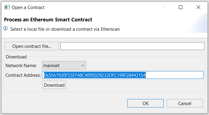
(*) Examples of code objects: a Windows PE file with x86-code, an ELF library with with MIPS code, a headless ARM firmware, a Wasm binary file, an Ethereum smart contract, etc.
Two important JEB API components to hook into and customize the native analysis pipeline are: – The IR classes – The AST classes We will start looking at IR components through the rest of this part 1.
IR Description
JEB IR can be seen as a low-level, imperative assembly language, made of expressions. Highest-level expressions are statements. Statements contain expressions. Generally, expressions can contain expressions. IR can be accessed via interfaces in the JEB API. The top-level interface for all IR expressions is IEGeneric. All IR elements start with IExxx. 2
The diagram below shows the current hierarchy of IR expression interfaces:
Note that IEGeneric sits at the top. All other IRE’s (short for IR Expressions from now on) derive from it. Let’s go through those interfaces:
IEImm: Integer immediate of arbitrary length. Eg, Imm(0x1122, 64) would represent the 64-bit integer value 0x1122.
IEVar: Generic IRE to represent variables. Variables can represent underlying physical registers, virtual registers, local function variables, global program variables, etc.
IEMem: Piece of memory of arbitrary length. The memory address itself is an IRE; the accessed bitsize is not.
IECond: A ternary expression “c ? a: b”, where a, b and c are IRE’s.
IERange: A fixed integer range, commonly used with Slice
IESlice: A chunk (contents range) of an existing IR. Eg, Slice(Imm(0x11223344, 32), 16, 24)) can be simplified to Imm(0x22, 8)
IECompose: The concatenation of two or more IRE’s (IR0, IR1, …), resulting in an IR of size SUM(i=0->n, bitsize(IRi))
IEOperation: A generic operation expression, with IRE operands and an operator. Eg, Operation(ADD,Imm(0x10,8),Mem(Imm(0x10000,32),8)). Most standard operators are supported, as well as less standard operators such as the Parity function or Carry function.)
IEStatement: the super-interface for IR statements; we will detail them below.
An IR translation unit, resulting from the conversion of a native routine, consists of a sequential list of IEStatement objects. An IR statement has a size (generally, but not necessarily, 1) and an address (generally, a 0-based offset relative to its position in the translation unit).
As of JEB 3.0.8, IR statements can be:
IEAssign: The most common of all statements: an assignment from a right-side source to a left-side destination. While the source can be virtually anything, the destination IRE is restricted to a subset of expressions.
IENop: This statement does nothing but consumes virtual size in the translation unit.
IEJump: An unconditional or conditional jump within the translation unit, expressed using IR offsets.
IEJumpFar: An unconditional or conditional far jump (can be outside the translation unit), expressed using native addresses.
IECall: Represent a well-formed static or dynamic dispatch to another IR translation unit. The dispatch expression can be any IRE (eg, an Imm for a static dispatch; a Var or Mem for a dynamic dispatch).
IEReturn: A high-level expression used to denote a return-to-caller from a translation unit representing a routine. This IRE is always introduced by later optimization passes.
IEUntranslatedInstruction: This powerful statement can be used to express anything. It is generally used to represent native instructions that cannot be readily translated using other IR expressions. (Users may see it as an IECall on steroid, using native addresses. In that sense, it is to IECall what IEJumpFar is to IEJump.)
Now, let’s look at a few examples of conversions.
IR Examples
Let’s assume the following EVars were previously defined by an Intel x86 (or x86-64) converter: tmp (a 32-bit EVar representing a virtual placeholder register); eax (an EVar representing the physical register %eax); ?f (1-bit EVars representing standard x86 flags).
x86: mov eax, 1
s32:_eax = s32:00000001h
Translating this mov instruction is straight-forward, and can be done with a single Assign IR statement.
x86-64: not r9d
s64:_r9 = C(~(s64:_r9[0:32[), i32:00000000h)
Translating a not-32-bit-register on an x86-64 platform is slightly more complex, as the upper 32-bit of the register are zeroed out. Here, the converter is making use of three nested IREs: (IECompose(IEOperation(NOT, Slice(r9, 0, 32))))
Reading IR.IECompose are pretty-printed as C(lo, …, hi), IESlice as Expr[m:n[
One side-effect of arithmetic operations on x86 is the modification of flag registers. A converter explicits those side effects. Consequently, translating the exclusive-or above resulted in several Assign IR statements to represent register and flags updates. 3
Reading IR. IEMem are pretty-printed as bitsize<SegmentIR>[AddressIR]
The translation of add makes use of the temporary, virtual EVar tmp. It holds the original value of %eax, before the addition was done. That value is necessary for some flag update computations (eg, the overflow flag.) Also take note of the use of special operators Parity and Carry in the converted stub.
Note that a native address is written to the RIP-IEVar (or any EVar representing the Program Counter – PC). PC-assignments like those can later be optimized to IEJump, making use of IR Offsets instead of Native Addresses.
Also note that the Control Flow Graph (CFG) of the native instruction in the examples thus far are isomorphic to their IR-CFG translated counterparts. That is not always the case, as seen in the example below.
Reading IR. conditional IEJump are pretty-printed “if (cond) goto IROffset”. Unconditional IEJump are rendered as simple “goto IROffset”.
This IR-CFG is not isomorphic to the native CFG. Additional edges (per the presence of 2x IEJump) are used to represent the compare “[esi+xxx] to [edi+xxx]” loop.
Accessing IR
The JEB back-end API allows full access to several IR-CFG’s, from low-level, raw IR to partially optimized IR, to fully lifted IR just before AST generation phases.
Navigating the IR in the GUI
The UI client currently provides access to the most optimized IR of routines. Those IR-CFG’s can be examined in the apt-named fragment right next to the source fragment showing decompiled code. Here is an example of a side-by-side assemblies (x86, IR). The next screenshot shows the decompiled source.
Left-side: x86 routine / Right-side: optimized IR of the converted routine (Click to enlarge)
Decompiled source
IR via API
The API is the preferred method when it comes to power-users wanting to manipulate the IR for specific needs, such as writing a custom optimizer, as we will see in the next blog in this series.
Reminder: JEB back-end plugins can be written in Java (preferably) or Python. JEB front-end scripts can be written in Python, and can run both in headless clients (eg, using the built-in command line client) or the UI client.
For now, let’s see how to write a Python script to:
Retrieve a decompiled routine
Get the generated Intermediate Representations
Print it out
The following script does retrieve the first internal routine of a Native unit, decompiles it, retrieve the default (latest) IR, and prints out its CFG. The full scripts is available on GitHub.
# retrieve `unit`, the code unit

# GlobalAnalysis is assumed to be on (default)
decomp = DecompilerHelper.getDecompiler(unit)
if not decomp:
  print('No decompiler unit found')
  return

# retrieve a handle on the method we wish to examine
method = unit.getInternalMethods().get(0)#('sub_1001929')
src = decomp.decompile(method.getName(True))
if not src:
  print('Routine was not decompiled')
  return
print(src)

decompTargets = src.getDecompilationTargets()
print(decompTargets)

decompTarget = decompTargets.get(0)
ircfg = decompTarget.getContext().getCfg()
# CFG object reference
# see package com.pnfsoftware.jeb.core.units.code.asm.cfg
print("+++ IR-CFG for %s +++" % method)
print(ircfg.formatSimple())
Running on Desktop Client. Run this script in the UI client via File, Scripts, Run… (hotkey: F3). Remember to open a binary file first, with a version of JEB that ships with the decompiler for that file’s architecture.
Running on the command-line. You may also decide to run it on the command-line. Example, on Windows:
That is it for part 1. In part 2, we will continue our exploration of the IR and see how we can hook into the decompilation pipeline to write our custom optimizers to clean packer-specific obfuscation, as well as make use of the data flow analysis components available with the IR-CFG. Stay tuned!
Working on IR presents several advantages, two of which being: a/ the reduction of coupling between the analysis pipeline and the input native architecture; b/ and offering a side-effect free representation of a program. ↩
The design choices of JEB IR are out-of-scope for this blog. They may be the subject of a separate document. ↩
When decompiling routines, IR optimization passes will iteratively refactor and clean-up unnecessary operations. In practice, most flag assignments will end up being removed or consolidated. ↩
Update: March 8, 2022: – The most up-to-date version of this document can be found in the Manual Update: Dec 8, 2021: – Reference section with list of special translations for EVM opcodes
Update: Jan 2, 2019:
– The full EVM decompiler shipped with JEB 3.0-beta.8
– Download a sample JEB Python script showing how to use the API Update: Nov 20, 2018: – We uploaded the decompiled code of an interested contract, the second part of the PolySwarm challenge (a good write-up can be found here)
We’re excited to announce that the pre-release of our Ethereum smart contract decompiler is available. We hope that it will become a tool of choice for security auditors, vulnerability researchers, and reverse engineers examining opaque smart contracts running on Ethereum platforms.
Keep on reading to learn about the current features of the decompiler; how to use it and understand its output; its current limitations, and planned additions.
This opaque multisig wallet is holding more than USD $22 million as of 10/26/2018 (on mainnet, address 0x3DBB3E8A5B1E9DF522A441FFB8464F57798714B1)
Overall decompiler features
The decompiler modules provide the following specific capabilities:
The EVM decompiler takes compiled smart contract EVM 1 code as input, and decompiles them to Solidity-like source code.
The initial EVM code analysis passes determine contract’s public and private methods, including implementations of public methods synthetically generated by compilers.
Code analysis attempts to determine method and event names and prototypes, without access to an ABI.
The decompiler also attempts to recover various high-level constructs, including:
Implementations of well-known interfaces, such as ERC20 for standard tokens, ERC721 for non-fungible tokens, MultiSigWallet contracts, etc.
Storage variables and types
High-level Solidity artifacts and idioms, including:
Function mutability attributes
Function payability state
Event emission, including event name
Invocations of address.send() or address.transfer()
Precompiled contracts invocations
On top of the above, the JEB back-end and client platform provide the following standard functionality:
The decompiler uses JEB’s optimizations pipeline to produce high-level clean code.
It uses JEB code analysis core features, and therefore permits: code refactoring (eg, consistently renaming methods or fields), commenting and annotating, navigating (eg, cross references), typing, graphing, etc.
Users have access to the intermediate-level IR representation as well as high-level AST representations though the JEB API.
More generally, the API allows power-users to write extensions, ranging from simple scripts in Python to complex plugins in Java.
Our Ethereum modules were tested on thousands of smart contracts active on Ethereum mainnet and testnets.
Basic usage
Open a contract via the “File, Download Ethereum Contract…” menu entry.
You will be offered two options:
Open a binary file already stored on disk
Download 2 and open a contract from one of the principal Ethereum networks: mainnet, rinkeby, ropsten, or kovan:
Select the network
Provide the contract 20-byte address
Click Download and select a file destination
Open a contract via the File, Open smart contract menu entry
Note that to be recognized as EVM code, a file must:
either have a “.evm-bytecode” extension: in this case, the file may contain binary or hex-encoded code;
or have be a “.runtime” or “.bin-runtime” extension (as generated by the solc Solidity compiler), and contain hex-encoded Solidity generated code.
If you are opening raw files, we recommend you append the “.evm-extension” to them in order to guarantee that they will be processed as EVM contract code.
Contract Processing
JEB will process your contract file and generate a DecompiledContract class item to represent it:
The Assembly view on the right panel shows the processed code.
To switch to the decompiled view, select the “Decompiled Contract” node in the Hierarchy view, and press TAB (or right-click, Decompile).
Right-click on items to bring up context menus showing the principal commands and shortcuts.
The decompiled view of a contract.
The decompiled contract is rendered in Solidity-like code: it is mostly Solidity code, but not entirely; constructs that are illegal in Solidity are used throughout the code to represent instructions that the decompiler could not represent otherwise. Examples include: low-level statements representing some low-level EVM instructions, memory accesses, or very rarely, goto statements. Do not expect a DecompiledContract to be easily recompiled.
Code views
You may adjust the View panels to have side-by-side views if you wish to navigate the assembly and high-level code at the same time.
In the assembly view, within a routine, press Space to visualize its control flow graph.
To navigate from assembly to source, and back, press the TAB key. The caret will be positioned on the closest matching instruction.
Side by side views: assembly and source
Contract information
In the Project Explorer panel, double click the contract node (the node with the official Ethereum Foundation logo), and then select the Description tab in the opened view to see interesting information about the processed contract, such as:
The detected compiler and/or its version (currently supported are variants of Solidity and Vyper compilers).
The list of detected routines (private and public, with their hashes).
The Swarm hash of the metadata file, if any.
The contract was identified as being compiled with Solidity <= 0.4.21
Commands
The usual commands can be used to refactor and annotate the assembly or decompiled code. You will find the exhaustive list in the Action and Native menus. Here are basic commands:
Rename items (methods, variables, globals, …) using the N key
Navigate the code by examining cross-references, using the X key (eg, find all callers of a method and jump to one of them)
Comment using the Slash key
As said earlier, the TAB key is useful to navigate back and forth from the low-level EVM code to high-level decompiled code
We recommend you to browser the general user manual to get up to speed on how to use JEB.
Rename an item (eg, a variable) by pressing the N key
Remember that you can change immediate number bases and rendering by using the B key. In the example below, you can see a couple of strings present in the bad Fomo3D contract, initially rendered in Hex:
All immediates are rendered as hex-strings by default.
Use the B key to cycle through base (10, 16, etc.) and rendering (number, ascii)
Understanding decompiled contracts
This section highlights idioms you will encounter throughout decompiled pseudo-Solidity code. The examples below show the JEB UI Client with an assembly on the left side, and high level decompiled code on the right side. The contracts used as examples are live contracts currently active Ethereum mainnet.
We also highlight current limitations and planned additions.
Dispatcher and public functions
The entry-point function of a contract, at address 0, is generally its dispatcher. It is named start() by JEB, and in most cases will consist in an if-statement comparing the input calldata hash (the first 4 bytes) to pre-calculated hashes, to determine which routine is to be executed.
JEB attempts to determine public method names by using a hash dictionary (currently containing more than 140,000 entries).
Contracts compiled by Solidity generally use synthetic (compiler generated) methods as bridges between public routines, that use the public Ethereum ABI, and internal routines, using a compiler-specific ABI. Those routines are identified as well and, if their corresponding public method was named, will be assigned a similar name __impl_{PUBLIC_NAME}.
NOTE/PLANNED ADDITION: currently, JEB does not attempt to process input data of public routines and massage it back into an explicit prototype with regular variables. Therefore, you will see low-level access to CALLDATA bytes within public methods.
A dispatcher.
Below, see the public method collectToken(), which is retrieving its first parameter – a 20 byte address – from the calldata.
A public method reading its arguments from CALLDATA bytes.
Interface discovery
At the time of writing, implementation of the following interfaces can be detected: ERC20, ERC165, ERC721, ERC721TokenReceiver, ERC721Metadata, ERC721Enumerable, ERC820, ERC223, ERC777, TokenFallback used by ERC223/ERC777 interfaces, as well as the common MultiSigWallet interface.
Eg, the contract below was identified as an ERC20 token implementation:
This contract implements all methods specified by the ERC20 interface.
Function attributes
JEB does its best to retrieve:
low-level state mutability attributes (pure, read-only, read-write)
the high-level Solidity ‘payable’ attribute, reserved for public methods
Explicitly non-payable functions have lower-level synthetic stubs that verify that no Ether is being received. They REVERT if it is is the case. If JEB decides to remove this stub, the function will always have an inline comment /* non payable */ to avoid any ambiguity.
The contract below shows two public methods, one has a default mutability state (non-payable); the other one is payable. (Note that the hash 0xFF03AD56 was not resolved, therefore the name of the method is unknown and was set to sub_AF; you may also see a call to the collect()’s bridge function __impl_collect(), as was mentioned in the previous section).
Two public methods, one is payable, the other is not and will revert if it receives Ether.
Storage variables
The pre-release decompiler ships with a limited storage reconstructor module.
Accesses to primitives (int8 to int256, uint8 to uint256) is reconstructed in most cases
Packed small primitives in storage words are extracted (eg, a 256-bit storage word containing 2x uint8 and 1x int32, and accessed as such throughout the code, will yield 3 contract variables, as one would expect to see in a Solidity contract
Four primitive storage variables were reconstructed.
However, currently, accesses to complex storage variables, such as mappings, mappings of mappings, mappings of structures, etc. are not simplified. This limitation will be addressed in the full release.
When a storage variable is not resolved, you will see simple “storage[…]” assignments, such as:
Unresolved storage assignment, here, to a mapping.
Due to how storage on Ethereum is designed (a key-value store of uint256 to uint256), Solidity internally uses a two-or-more indirection level for computing actual storage keys. Those low-level storage keys depend on the position of the high level storage variables. The KECCAK256 opcode is used to calculate intermediate and final keys. We will detail this mechanism in detail in a future blog post.
Precompiled contracts
Ethereum defines four pre-compiled contracts at addresses 1, 2, 3, 4. (Other addresses (5-8) are being reserved for additional pre-compiled contracts, but this is still at the ERC stage.)
JEB identifies CALLs that will eventually lead to pre-compiled code execution, and marks them as such in decompiled code: call_{specific}.
The example below shows the __impl_Receive (named recovered) method of the 34C3 CTF contract, which calls into address #2, a pre-compiled contract providing a fast implementation of SHA-256.
This contract calls address 2 to calculate the SHA-256 of a binary blob.
Ether send()
Solidity’s send can be translated into a lower-level call with a standard gas stipend and zero parameters. It is essentially used to send Ether to a contract through the target contract fallback function.
NOTE: Currently, JEB renders them as send(address, amount) instead of address.send(amount)
The contract below is live on mainnet. It is a simple forwarder, that does not store ether: it forwards the received amount to another contract.
This contract makes use of address.send(…) to send Ether
Ether transfer()
Solidity’s transfer is an even higher-level variant of send that checks and REVERTs with data if CALL failed. JEB identifies those calls as well.
NOTE: Currently, JEB renders them as transfer(address, amount) instead of address.transfer(amount)
This contract makes use of address.transfer(…) to send Ether
Event emission
JEB attempts to partially reconstruct LOGx (x in 1..4) opcodes back into high-level Solidity “emit Event(…)”. The event name is resolved by reversing the Event method prototype hash. At the time of writing, our dictionary contains more than 20,000 entries.
If JEB cannot reverse a LOGx instruction, or if LOG0 is used, then a lower-level log(…) call will be used.
NOTE: currently, the event parameters are not processed; therefore, the emit construct used in the decompiled code has the following form: emit Event(memory, size[, topic2[, topic3[, topic4]]]). topic1 is always used to store the event prototype hash.
An Invocation of LOG4 reversed to an “emit Deposit(…)” event emission
API
JEB API allows automation of complex or repetitive tasks. Back-end plugins or complex scripts can be written in Python or Java. The API update that ship with JEB 3.0-beta.6 allow users to query decompiled contract code:
access to the intermediate representation (IR)
access to the final Solidity-like representation (AST)
API use is out-of-scope here. We will provide examples either in a subsequent blog post or on our public GitHub repository.
Additional References
List of EVM opcodes that receive special translation: link (on GitHub)
Conclusion
As said in the introduction, if you are reverse engineering opaque contracts (that is, most contracts on Ethereum’s mainnet), we believe you will find JEB useful.
You may give a try to the pre-release by downloading the demo here. Please let us know your feedback: we are planning a full release before the end of the year.
As always, thank you to all our users and supporters. -Nicolas
We published a paper deep-diving into WebAssembly from a reverse engineer point of view (wasm format, bytecode, execution environment, implementation details, etc.).
The paper annex details how JEB can be used to analyze and decompiler WebAssembly modules.
Code and decompilation view of a WebAssembly module
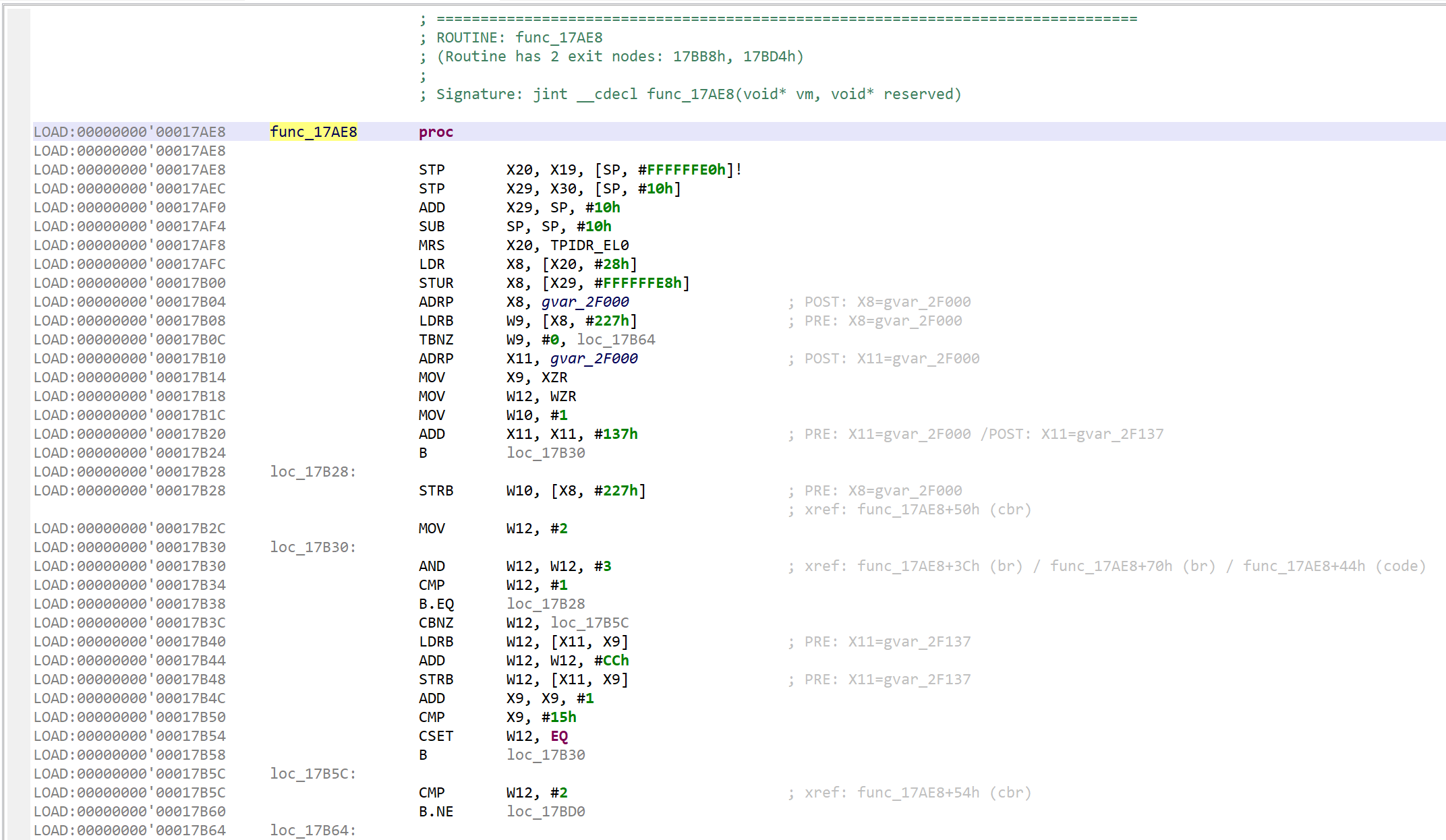
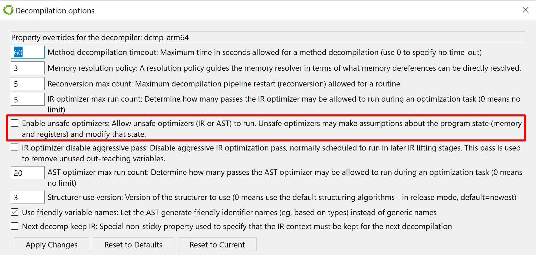
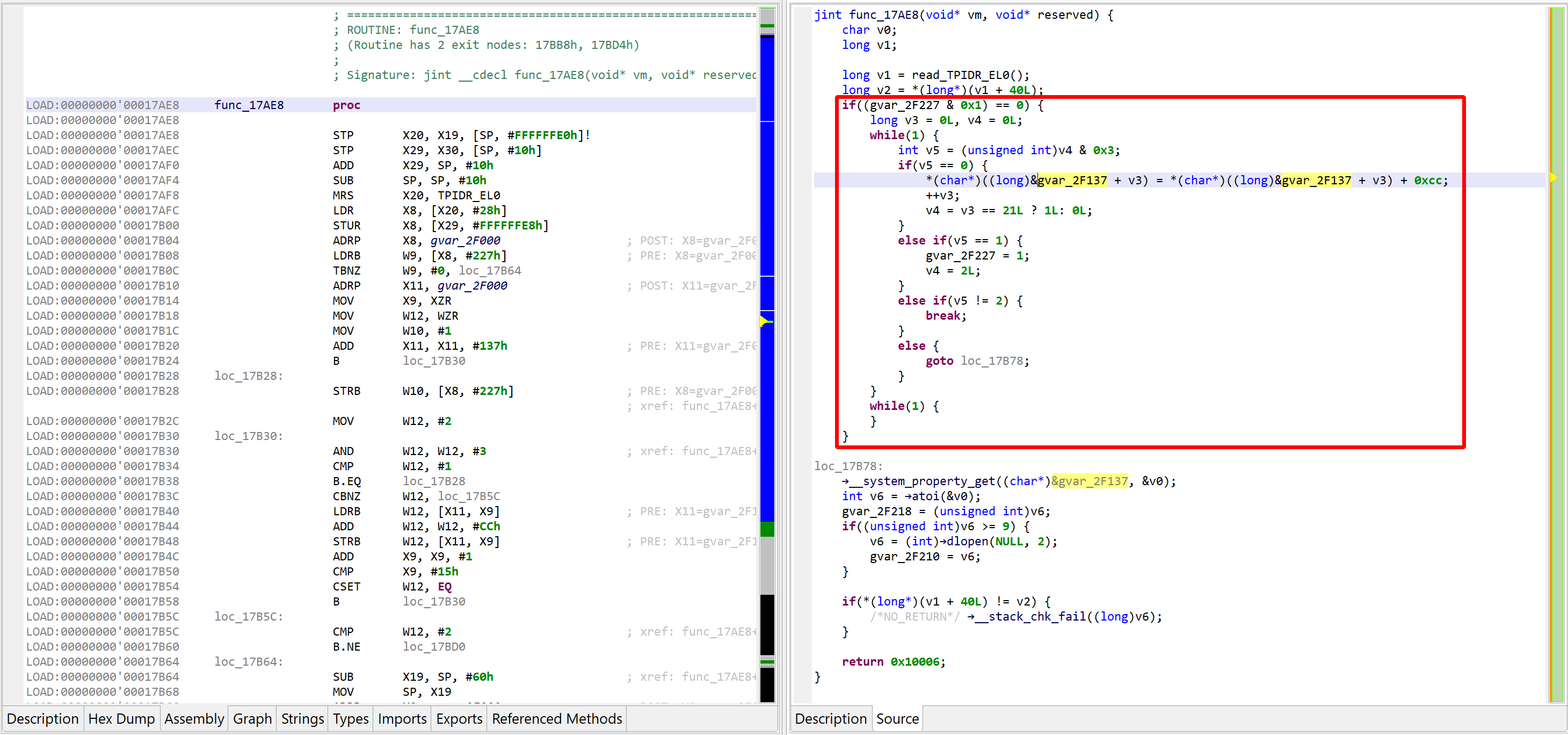
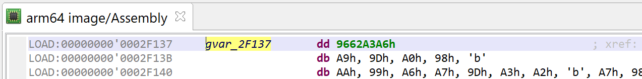
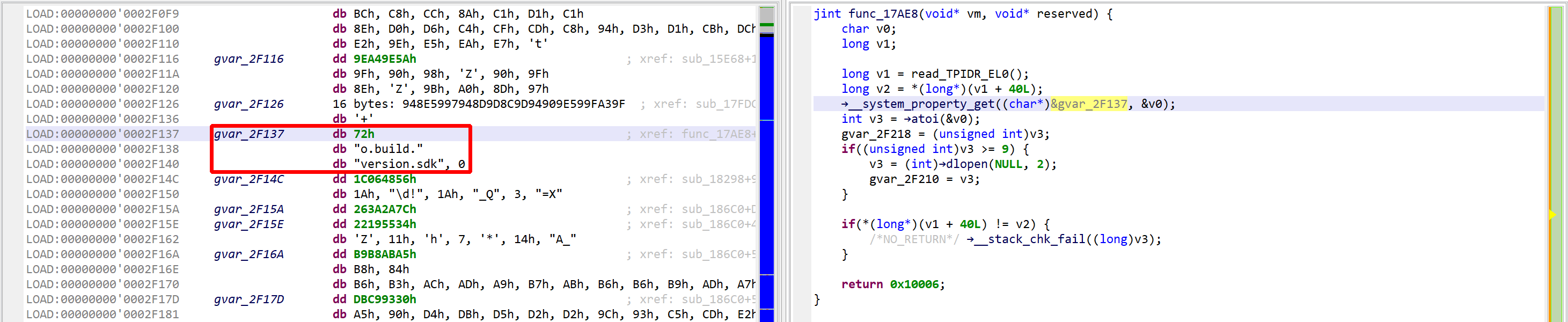
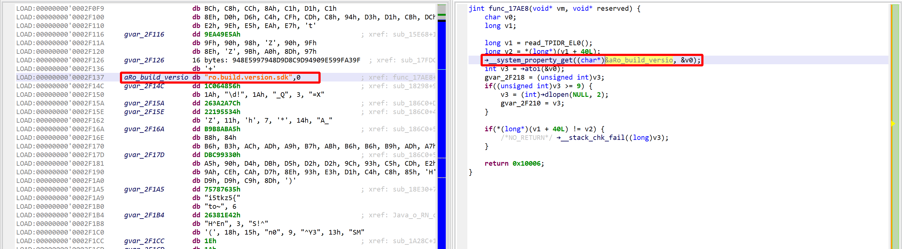
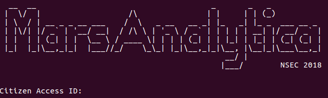
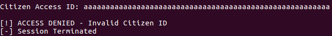
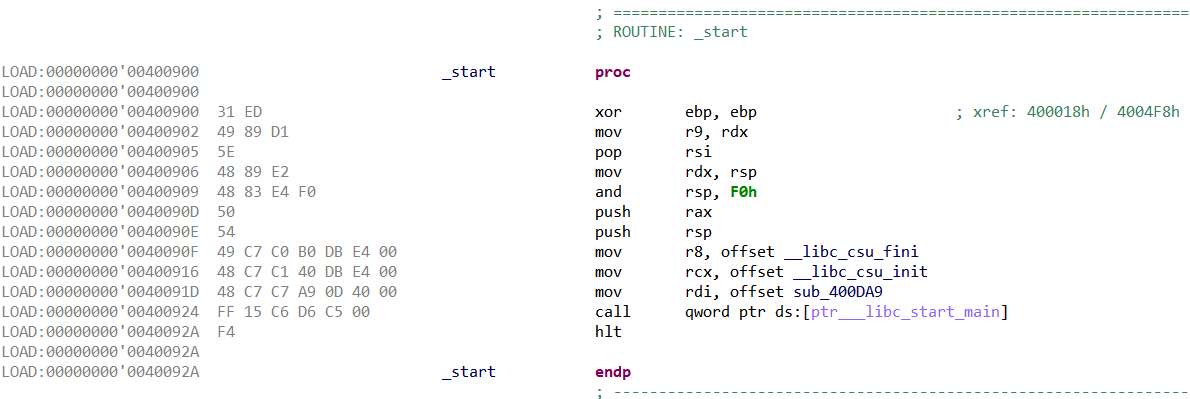
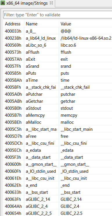
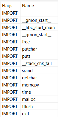

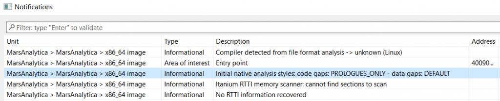
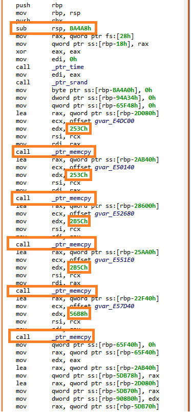
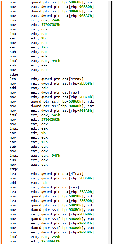
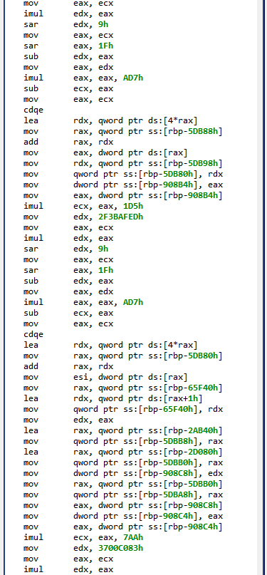
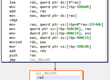
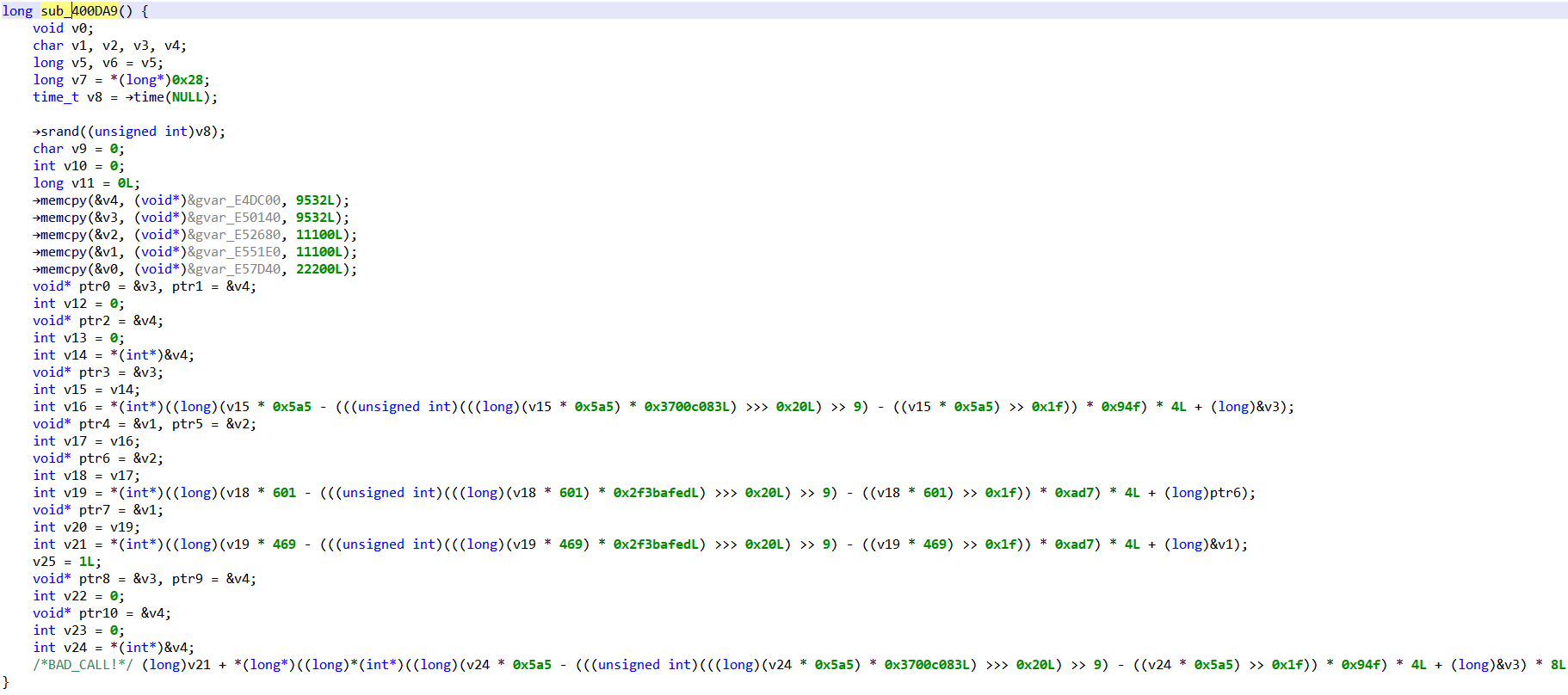
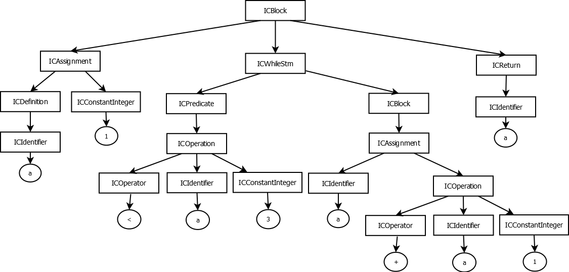
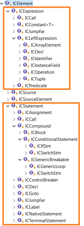
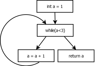
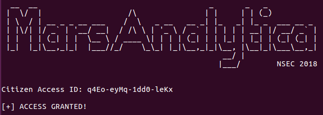
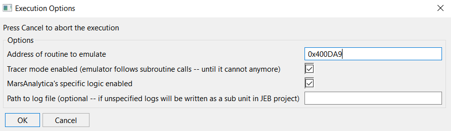
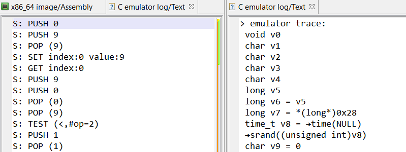
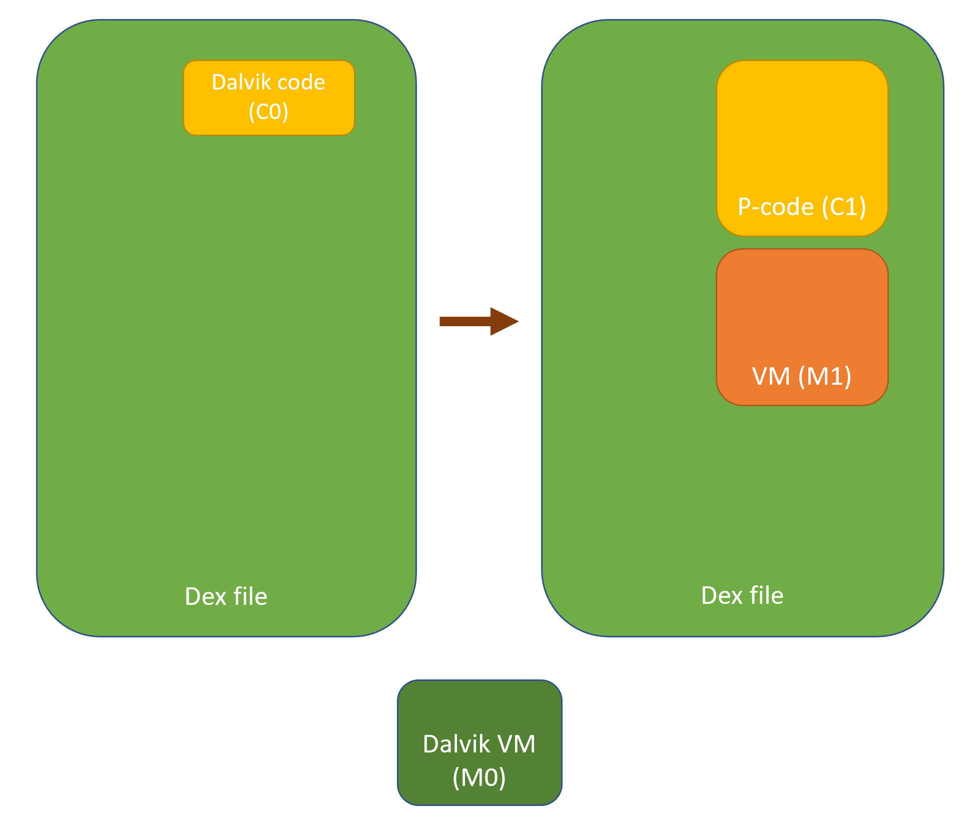
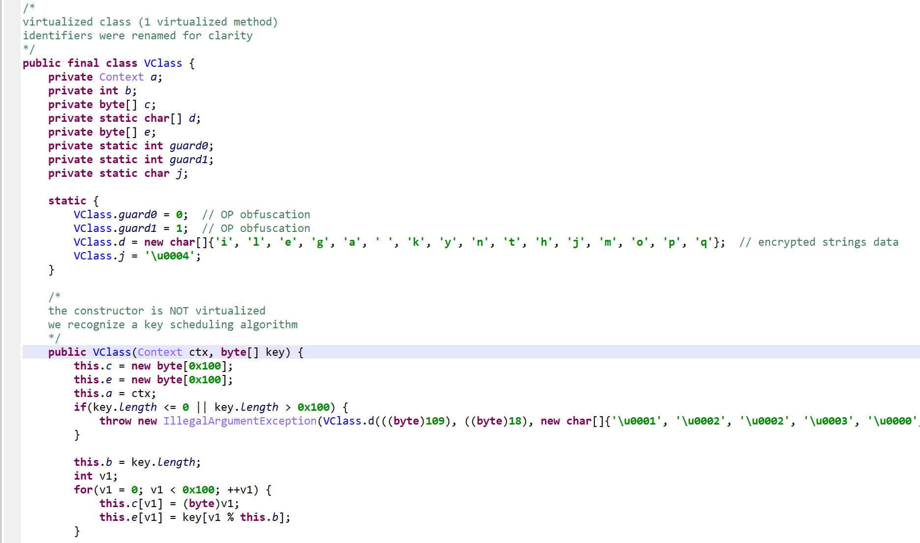
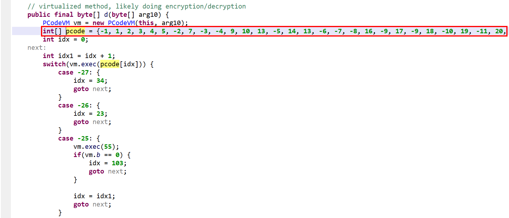
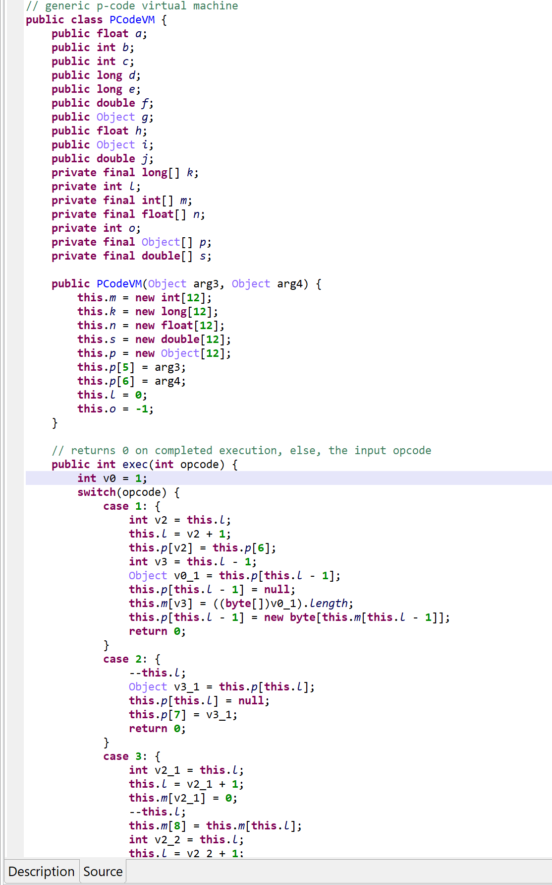


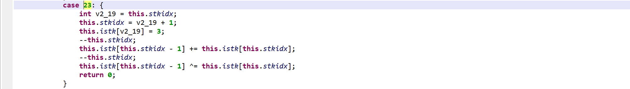
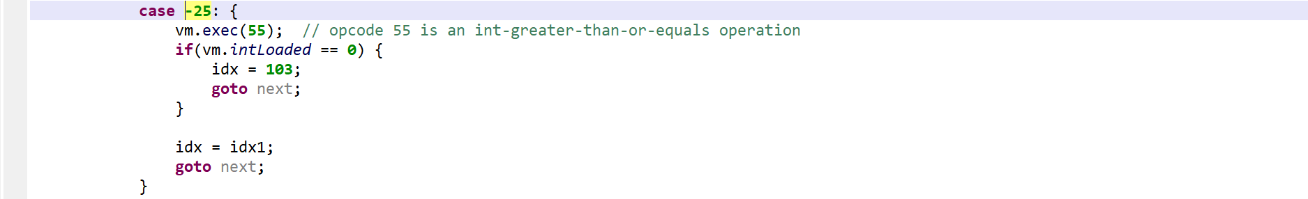
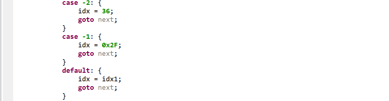


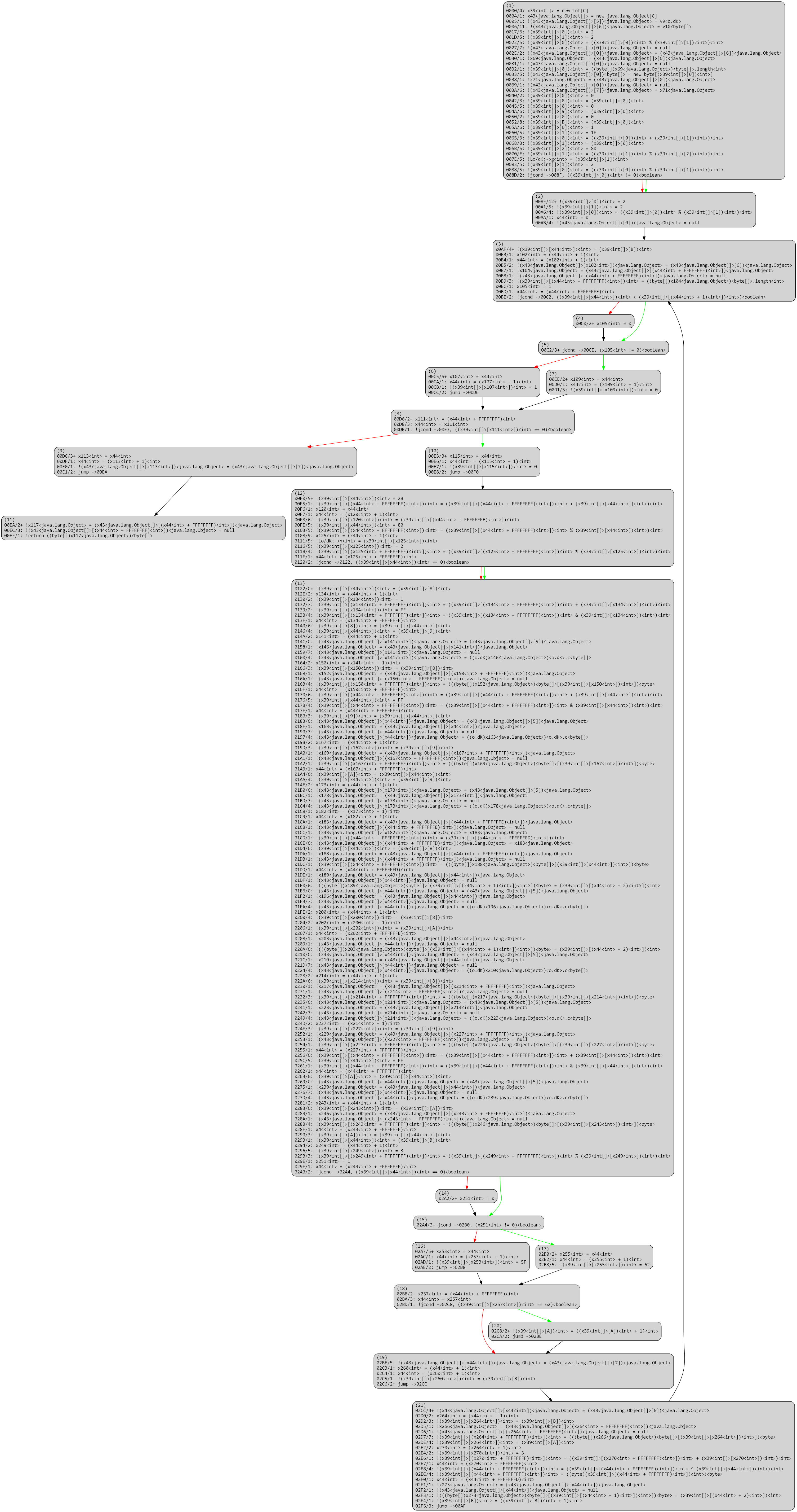
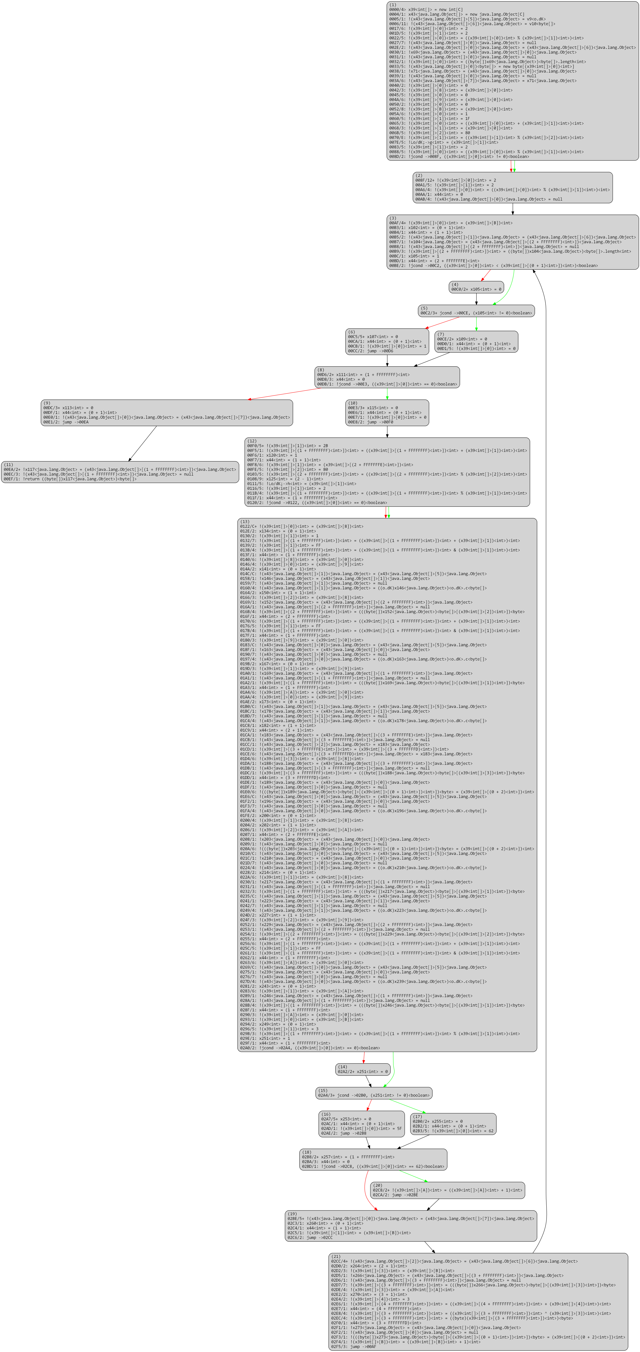
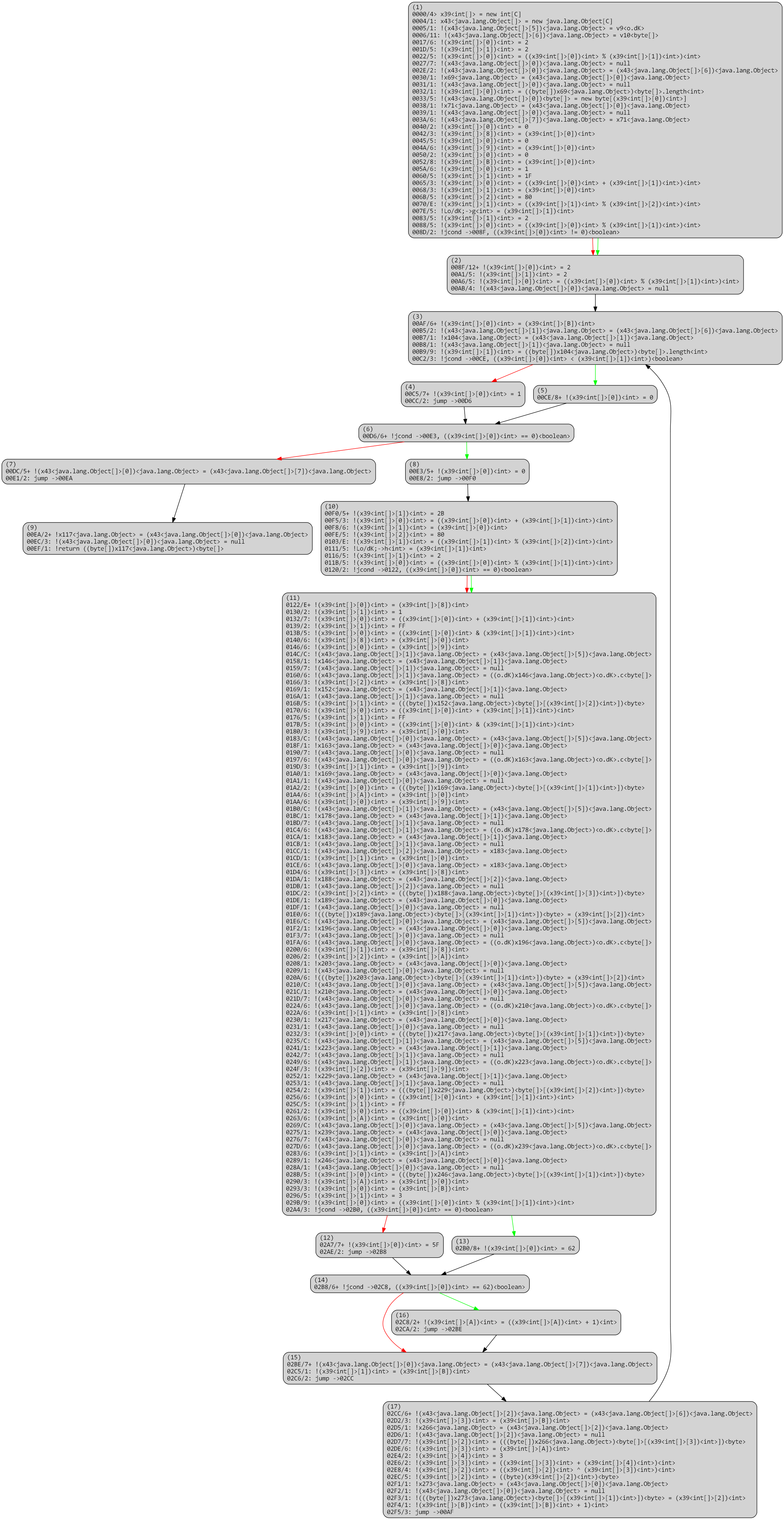
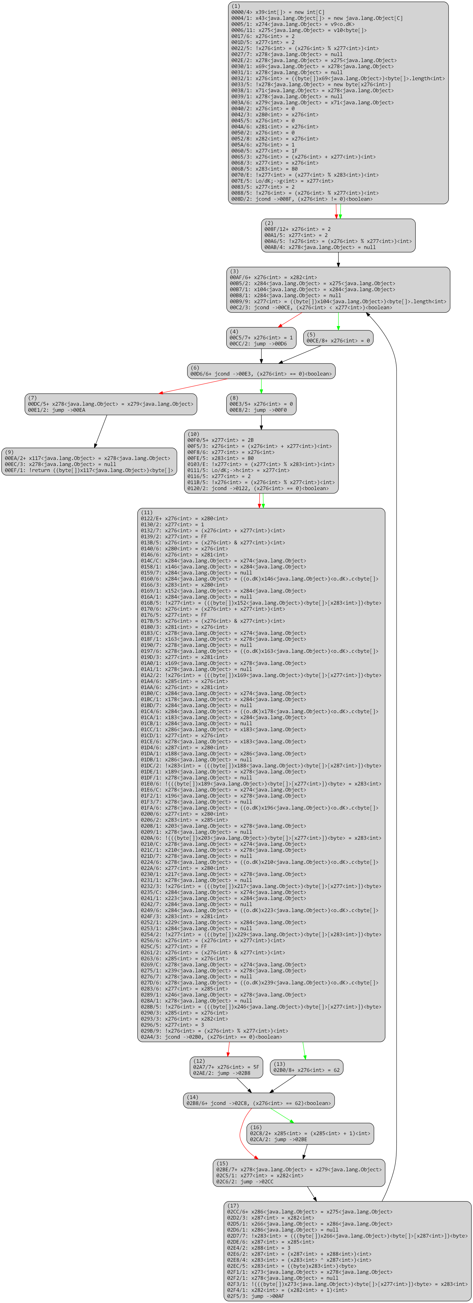
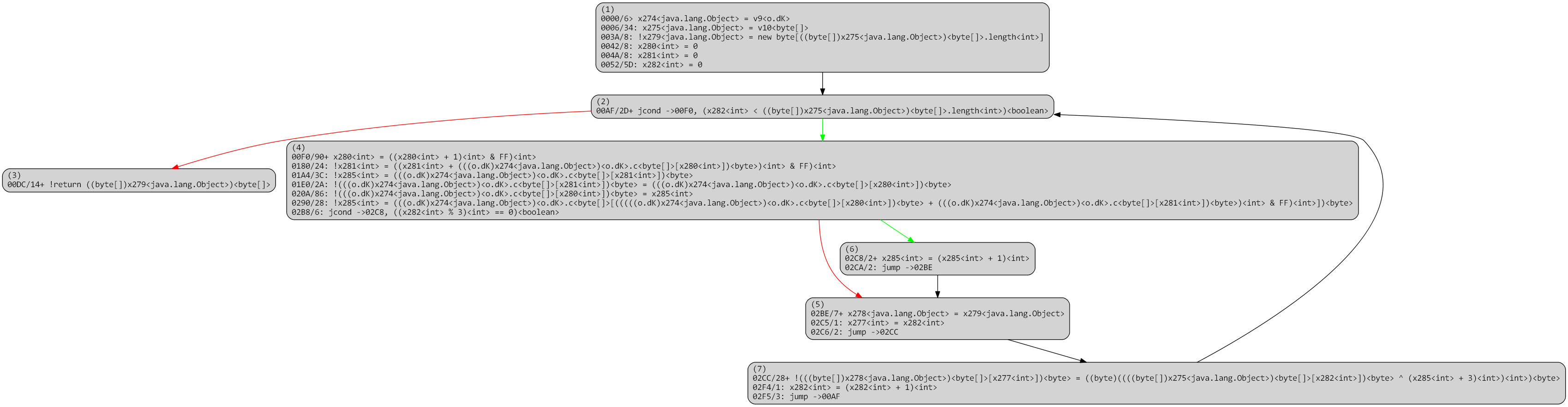
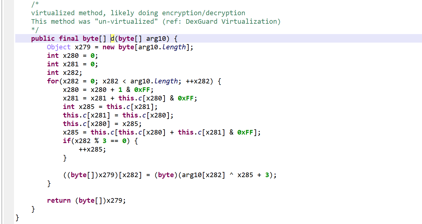
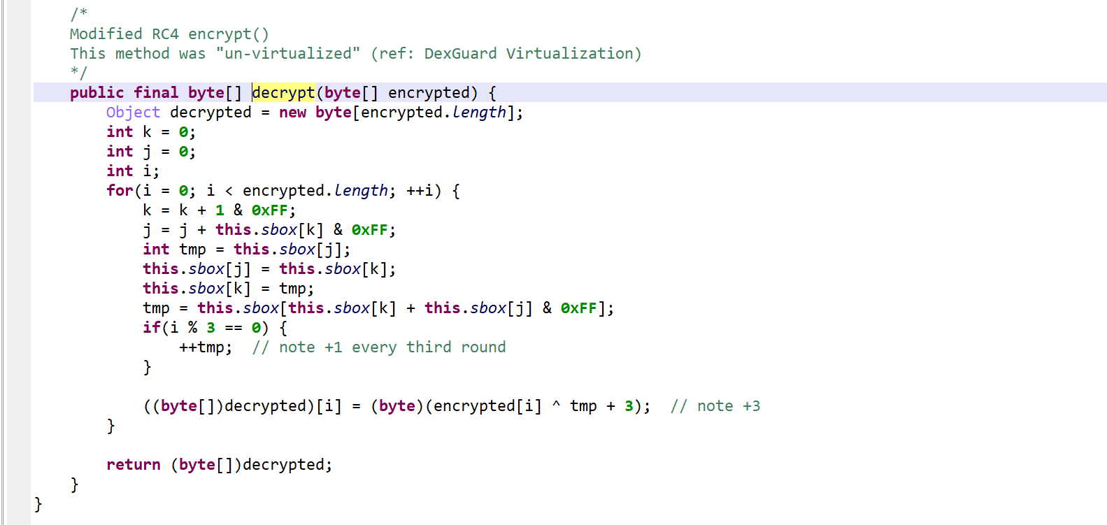
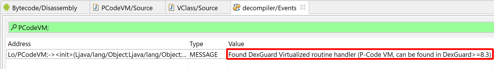
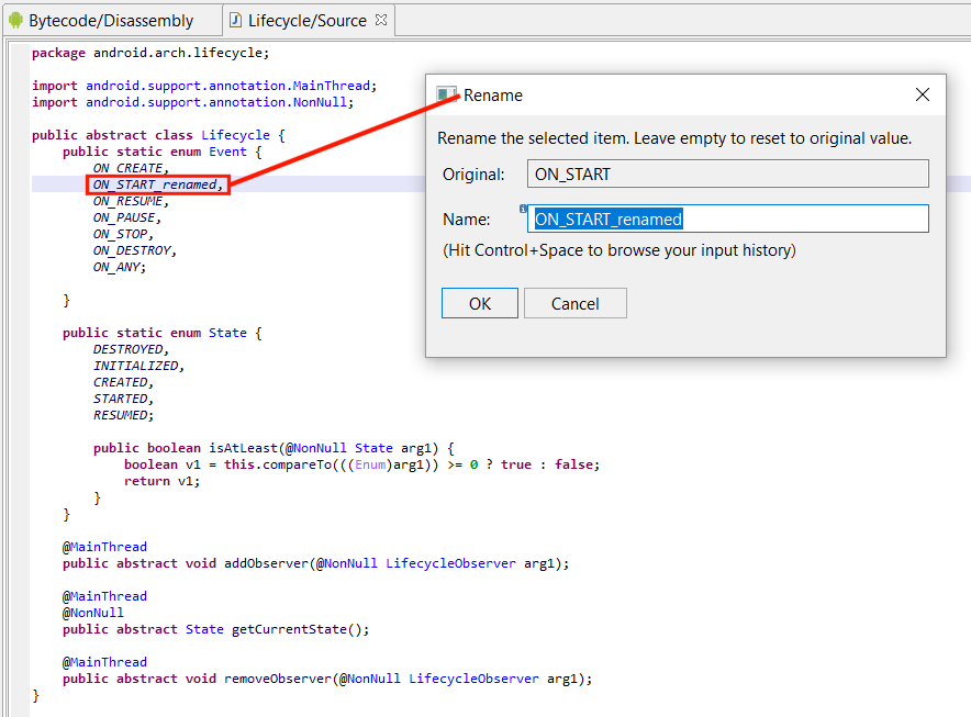
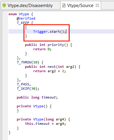
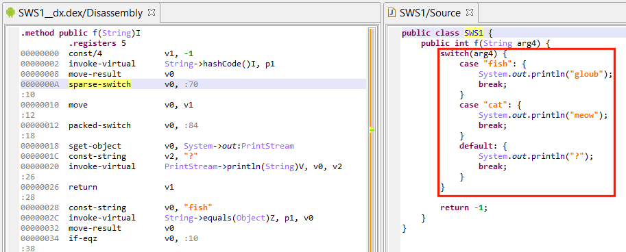
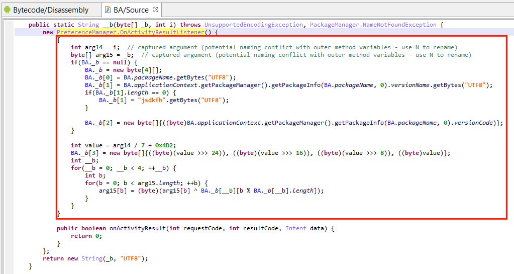
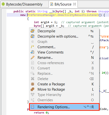
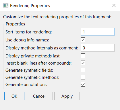
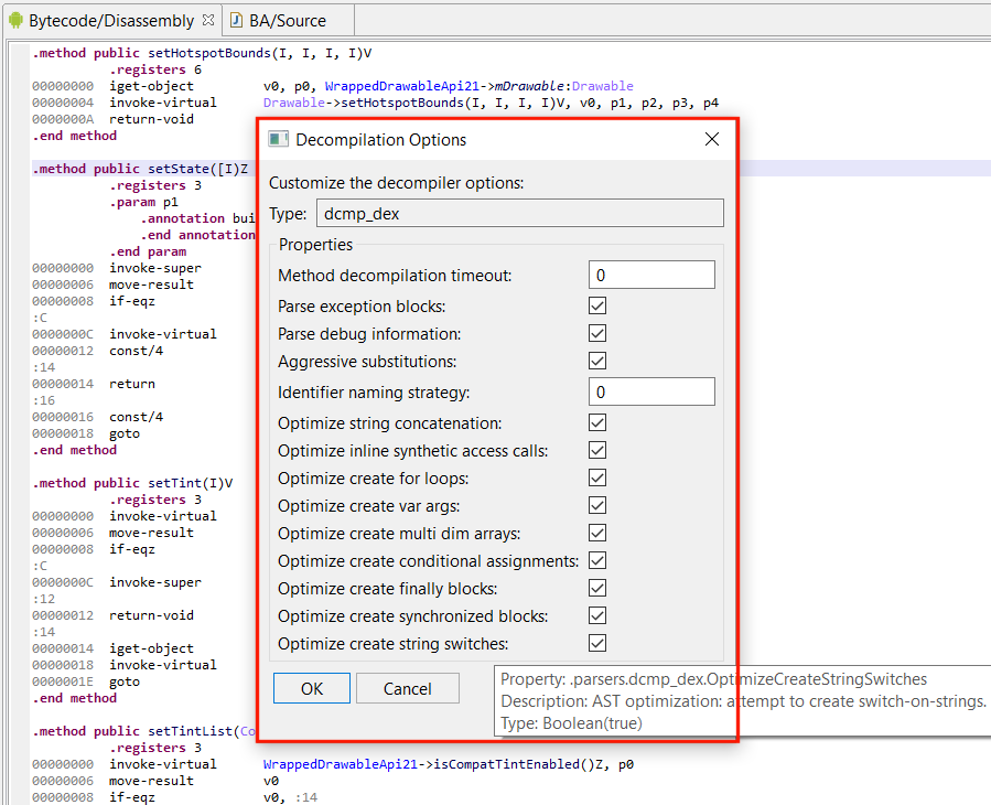
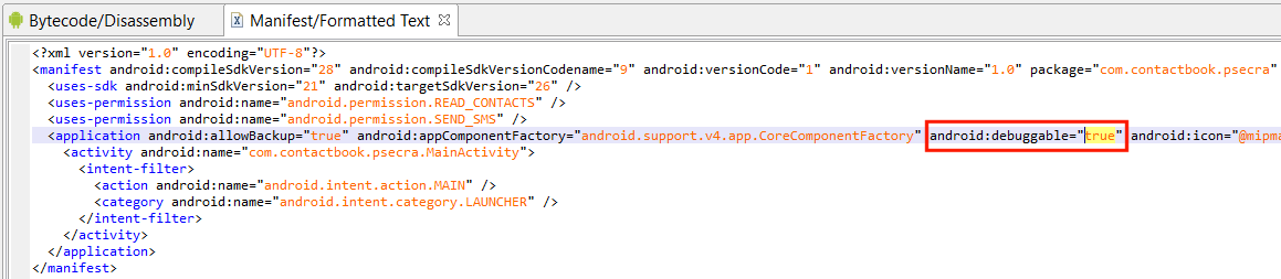
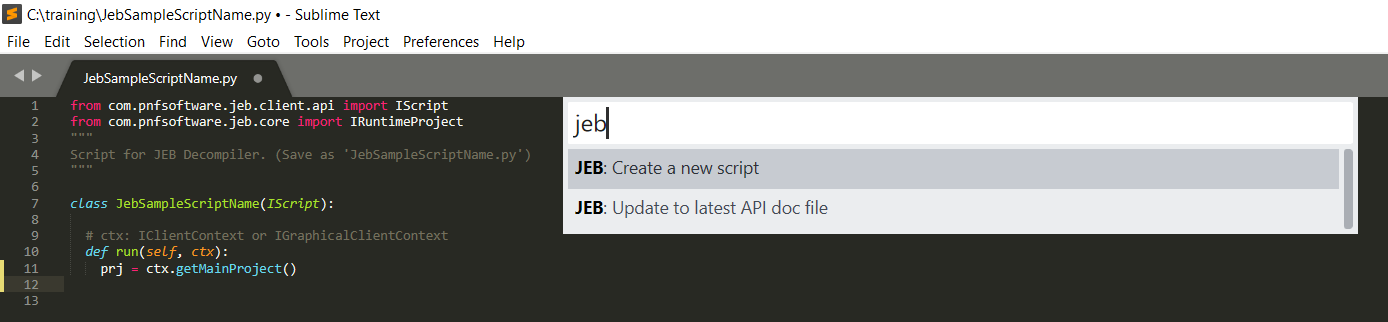
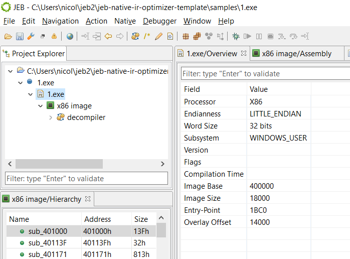
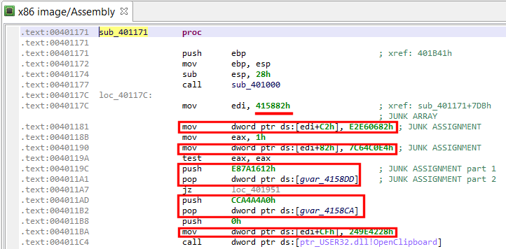
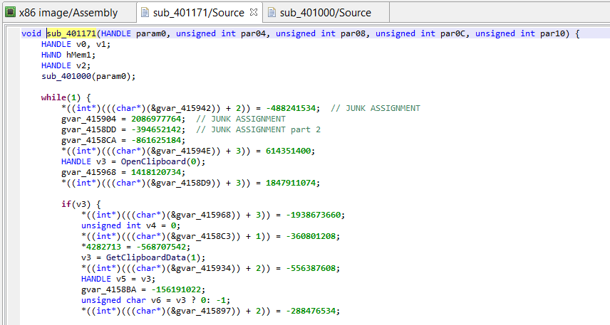
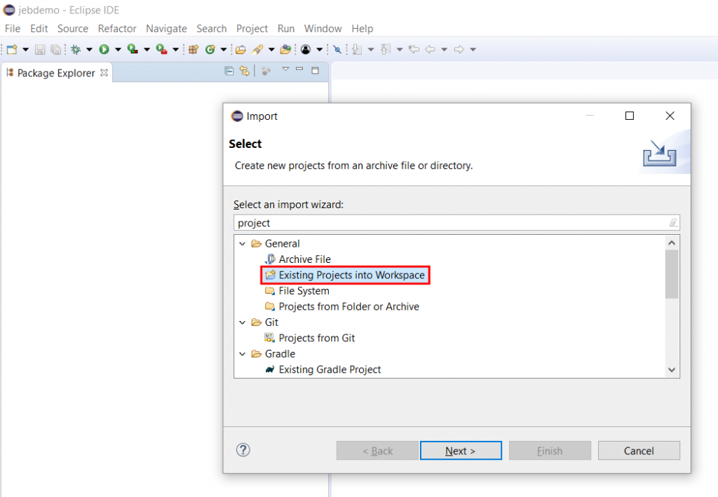
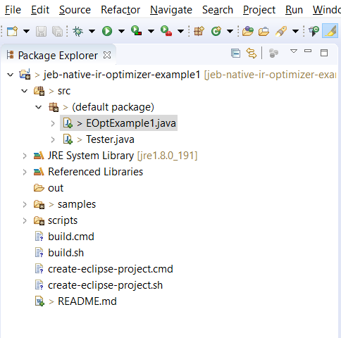
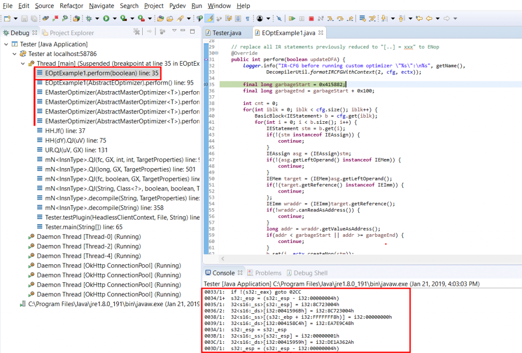
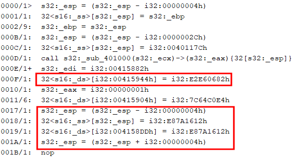
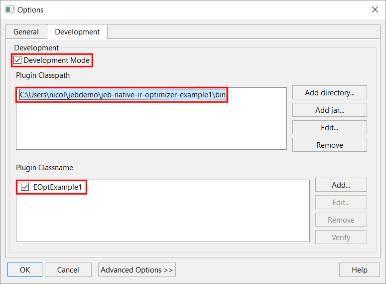
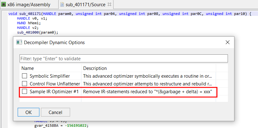
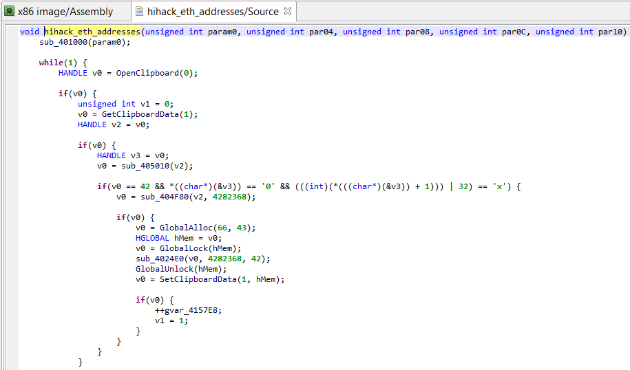
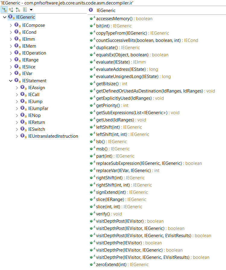
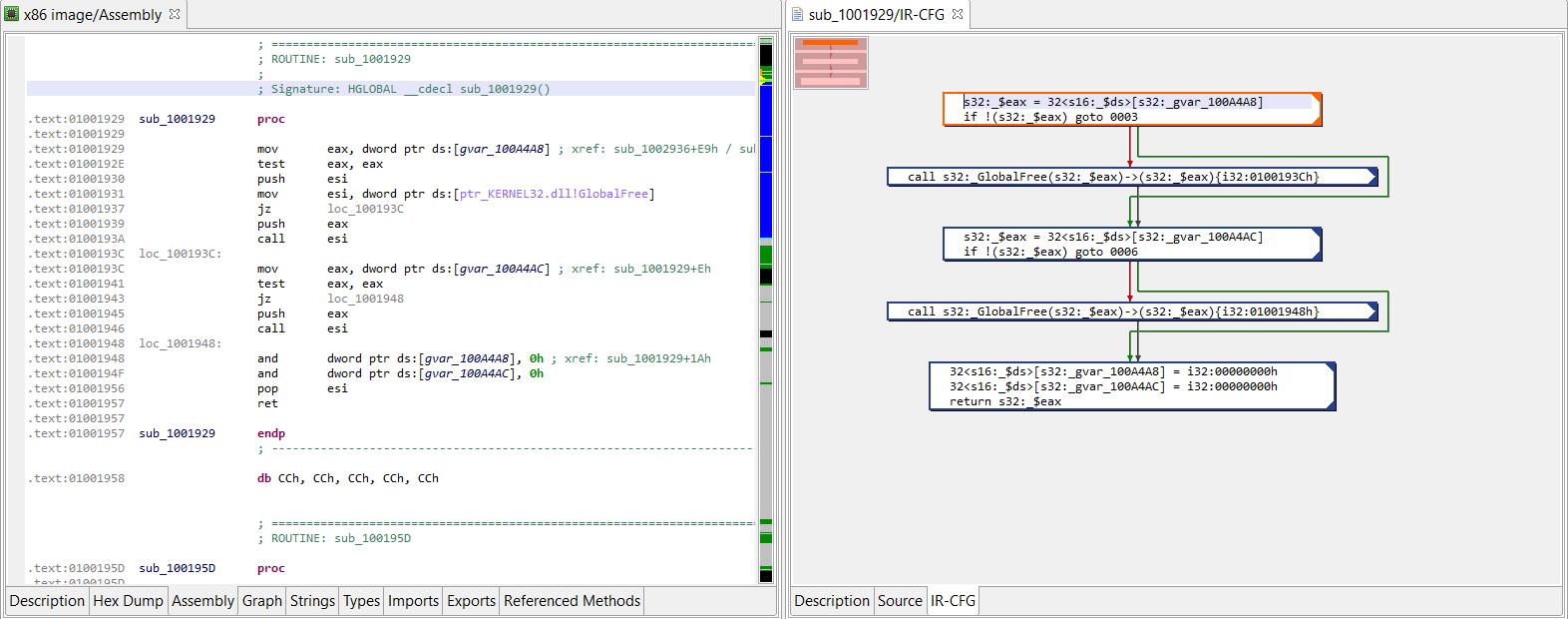
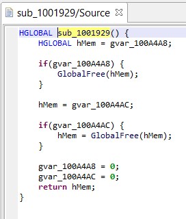
 We’re excited to announce that the pre-release of our Ethereum smart contract decompiler is available. We hope that it will become a tool of choice for security auditors, vulnerability researchers, and reverse engineers examining opaque smart contracts running on Ethereum platforms.